Killing Model-Based Control Dead Time

Model-based control was introduced as a method of achieving a setpoint response that emulated open-loop response, thereby eliminating the overshoot and cycling commonly experienced under PID control. It is also ideal for dead-time-dominant processes such as paper machines. If there is no exponential lag in the path of the load disturbance, it also provides satisfactory load regulation.
Its limitation is that the lag-dominant processes commonly encountered in fluid processing have the same dominant exponential lag in the path of the load disturbance as in the path of the controller output. This results in a slow exponential recovery following a step load change. The limitation imposed by these "disturbance dynamics" was previously explained by the author in some detail in Control.
The reason for the slow exponential recovery is the use of the model to estimate the load change and match it with an identical change in controller output. The appearance of open-loop control predominates in load response, just as it does in response to setpoint changes. Much faster load response is achievable if the manipulated variable is made to overshoot the load change. The amount of overshoot that produces the best response varies with the ratio of dead time to the exponential lag.
Here we define the best load response (regulation) for a first-order-plus-dead-time process, and examine the possibility of approaching it. While real fluid processes are more complex, the behavior of this fundamental model is very easy to visualize and forms a basis for understanding what is possible using real controllers on real processes.
Dead-Time Dominance
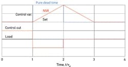
This pure dead-time process is easy enough to understand. A step in load produces a step in the controlled variable one dead time later. A model-based controller will respond by stepping its output an amount equal to the load step as estimated through the model. If the two changes are indeed matched, the controlled variable will return to setpoint following the next dead time. Figure 1 shows the best response to a step load change for the pure dead-time process having a steady-state gain of 2.0 (in blue)—a load step of 10% produces a deviation of 20%, which the controller converts to an output step of 10% to eliminate the deviation one dead time later.
The limitation encountered here is model mismatch, which has two dimensions: gain and time. If the model gain is too low, the loop gain is < 1, and return to setpoint will follow a series of decaying exponential steps; if too high, recovery will follow a cycle having a period of two dead times, damped if the loop gain is < 2. A dynamic mismatch is more serious, producing harmonic vibrations. To increase robustness and dampen any harmonics, filtering or sampling are generally applied, both of which reduce performance, as they effectively add to the loop dead time.
Pure dead-time fluid processes are uncommon, but static mixers can be dead-time-dominant. Their lags filter out potential harmonics, but also make control more difficult. Of more consequence here is the pursuit of best regulation for lag-dominant processes.
Non-Self-Regulating (NSR) Processes
Dead-time and integrating processes
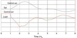
Figure 1. Best step-load responses for a dead-time and an integrating (NSR) process.
Following a step change in load (inflow for example), the level will ramp during the following dead time, as shown in the red trace of Figure 1. Control action can't begin until the level starts to change, and it can have no effect until another dead time elapses. The best regulator for a non-self-regulating (NSR) process would step its output as soon as the controlled variable deviates from setpoint. But, stepping it an amount equal to the estimated load step would leave the level offset by the amount it changed during the dead-time interval between the two steps. To eliminate any offset, the step in controller output must overshoot the load step. Figure 1 shows the best response, attained by the controller output doubling the load step, followed by a matching of the load at the end of the next dead time.
This best response curve is identified by two characteristics: its peak deviation, eb (reached after one dead time), and Integrated Error, IEb. Both have economic consequences: Peak deviation determines how closely the setpoint can be positioned to operating constraints such as trip points, and IE is a measure of excess energy use or product giveaway. Both should be minimized, and they are related. For the NSR process:
eb = ∆qτd/τ (1)
IEb = ebτd = ∆qτd2/τ (2)
where ∆q is the size of the load change; τd is the loop dead time; and τ is the integrating time constant of the process. (In Figure 1, the controlled variable changed twice as much as the load during the dead time, so the integrating time of this process is one-half the dead time.) Note that IEb varies with the square of the dead time. With a real controller, peak deviation will be larger and occur later, with a resulting much higher IE.
Manipulated-variable overshoot is essential in achieving a prompt and complete return to setpoint. However, the approach to this best load regulation is hindered in two ways. The output step must be initiated at the earliest detection of a deviation to achieve earliest recovery, and information obtained at that time is least accurate in estimating the required size of the output step. Based on the ramp rate of the level, the step size can be more accurately estimated with time. Then, when the direction of the level finally changes, the overshoot must be promptly removed, with a similar demand on accuracy.
No controller has the accuracy required to do this. Secondly, the derivative action needed to determine ramp rate can't be applied to level measurements due to its sensitivity to noise. So we're limited to PI control of liquid level (with feed-forward as necessary with boiler-drum applications). But the tuning of the PI controller should reflect the output motion that resembles the best, 100% output overshoot being an essential feature.
Self-Regulating Processes
Most processes are self-regulating, having a proportional relationship between the controlled and manipulated variables. Model-based controllers relate the two to predict the result of output moves, but typically provide no output overshoot for prompt recovery from load changes. Only pure dead-time processes require no output overshoot for best response. For all others, the size of the output step in relation to the load step follows the equation below (derived in Reference 2 in my book, Process Control Systems, 4th ed., McGraw-Hill, New York, 1996, p. 35):
∆m/∆q = 1+ετd/τ1 (3)
where ∆m and ∆q are the changes in manipulated variable and load respectively; τd is dead time in the loop; τ1 is the time lag in the load path; and ε is 2.718, the base of natural logarithms. At the end of the following dead time, m and q would be set equal.
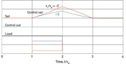
Figure 2 shows best load responses for two lag-dominant processes: a self-regulating process in blue, and an unstable process in red, to be described later. Their required output overshoots both follow the above equation.
Peak deviation for the stable (self-regulating) process is
εb = ∆qKp(1-e-τd/τ1) (4)
where Kp is the process steady-state gain, having a value of 2.0 in this example; and τ1 is its exponential lag time. The departure and recovery curves are complementary, so that IEb = ebτd as before. In Figure 2, τ1 is twice τd, requiring a peak output/load ratio of 1.607, or 60.7% overshoot. Most lag-dominant processes feature a τd/τ1 ratio of around 1/7, requiring an output/load ratio of 1.867 or 86.7% overshoot, approaching the 100% for NSR processes.
Unstable Processes
Tuning for overshoot
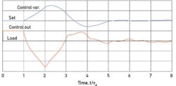
Figure 4. Minimum-IAE tuning of the PIDτ controller gives the requisite MV overshoot.
The manipulated-variable overshoot required for best load response follows Equation 3, as for the self-regulating process, but with the time constant being negative, the overshoot exceeds 100%, or 165% in this example.
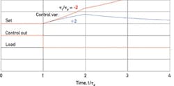
Figure 3 compares the load responses for the same two processes where no manipulated-variable (MV) overshoot is applied—typical of model-based control. The self-regulating process recovers in a long exponential curve, reflecting the time lag in the load path. In this example, its value is only two dead times, but it's more commonly around seven dead times, resulting in poor load regulation indeed.
But the absence of MV overshoot with the unstable process is catastrophic—temperature runaway! A familiar analog of an unstable process is the inverted pendulum—any disturbance will cause it to accelerate away from the vertical position. Attempting to balance an inverted pendulum on the hand will only be successful if the hand moves farther in correcting a deviation of the tip of the pendulum than the size of that deviation: Over 100% MV overshoot is essential in stabilizing an unstable process. But effective control is possible, as any trained seal can demonstrate.
This limitation is not inconsequential. Writing on the control of unstable petroleum hydrocracking reactors in "Update Hydrocracking Reactor Controls for Improved Reliability," Hydrocarbon Processing, October 2012, noted expert Allan Kern reports: "MPC [model-predictive control] is often considered a comprehensive solution for the type of control concerns raised here. However, none of the critical excursion control, depressure prevention or auto-quench functions are of the type provided by MPC."
Grading Real Controllers
The unstable process is especially demanding of regulators. Just as liquid-level loops can develop cycles when the controller's proportional band is too wide as well as too narrow, the unstable process can as well (See Process Control Systems, p. 320). If the dead time is sufficiently short relative to the lag time, an unstable process like a stirred-tank reactor can be regulated under proportional + integral (PI) control, but not the example considered here. No combinations of settings will be successful; derivative action (D) is essential.
Two candidates are now proposed for the unstable process described in Figures 2 and 3. The first to be considered adds dead-time compensation to the reset-feedback loop of a series-connected PID (interacting) controller, creating a PIDτ controller. Figure 4 describes its step-load response when tuned to minimize integrated absolute error (IAE). Its output cannot reproduce the step in load, but does overshoot it by 256% (compared to the best at 165%). The resulting peak deviation is only 1.14eb, reached 0.3 dead times later than the best. The IE of the response curve is about 18% higher than the best.
Along with its high performance comes limited robustness—the loop can destabilize if the process gain or dead time change in either direction. Yet the controller was successfully applied to a steam superheater in a 500-MW power boiler by gain-scheduling all four tuning parameters as a function of measured steam flow (See my "PID-Dead Time Control of Distributed Processes," Control Eng. Practice, 9(2001), 1177-1183).
Figure 4 also reveals a ripple in the controller output, which appears to decay—evidence of a "hot" controller. Secondary lags common to real processes will probably filter those out.
The more familiar alternative would be the ISA standard (non-interacting) PID controller (Figure 5). Its MV overshoot is 190%, causing deviation to peak at 1.25eb, reached 0.56 dead times later than the best. The IE of the response curve is also about 56% higher than IEb. While its performance is lower than the dead-time compensated PID, its robustness is higher by a factor of nearly three.
Conclusions
There are reasons why the PID controller continues to dominate the process-control field. It is not archaic or obsolete or simply a mathematical construct soon to be replaced by model-based control. Adding dead-time compensation improves its performance in the same way as it contributes to model-based control—and diminishes robustness for the same reasons, too. The success of high-level control loops for product quality and economic efficiency depends on a foundation of well-performing regulatory loops.
