Greg McMillan is a member of the Process Automation Hall of Fame (2001). Pierce Wu is a simulation project engineer at Mynah Technologies.
Simple and inexpensive inferential measurements of composition can be used to fill in the blanks. The inputs to the inferential measurements use common sensors, probes and meters that can be inserted in a line. The measurements are continuous and require no sample preparation. Except for spectral calculations, the computational time is less than a second so inferential measurements are essentially as fast as the sensors, probes and meters.
Inferential measurements must always be corrected at some point by analyzers and first-principle calculations. Consequently, the use of inferential measurements does not eliminate the need for analysis somewhere at some time. The analyzer could be in the field, a plant lab or a third-party lab.
Inferential measurements offer the ability to eliminate the considerable delay of at-line analyzers (e.g. 5-50 min) and excessive and variable delay of offline analyzers (e.g. 2 h to 2 wk) and reduce the vulnerability to analyzer resolution limits and failures. Inferential measurements also can eliminate process dead time and process time constants, providing an essentially instantaneous response with future values. The opportunities for expanding the scope and effectiveness of online data analytics and closed-loop control can be extraordinary.
Clue In on Step Response
Here we focus on the use of step-response models to provide a linear dynamic estimator. While the inputs are typically accurate mass flows, densities and temperatures, other online measurements of physical properties such as conductivity, dielectric spectroscopy, pH, turbidity and viscosity may be used. The ISA Interchange post "Inferential Measurements of Process Compositions" discusses practical considerations in the use of these physical property measurements.
Step response models can take advantage of the software used to identify the dynamics for tuning and for model predictive control (MPC). The process inputs that affect the inferential measurement are stepped in both directions, possibly with a pseudo-random binary sequence similar to what is done to identify the MPC dynamics of disturbance variables. The process outputs being predicted are analyzer measurements with the same cycle time and analysis time as during normal operation.
So that the MPC inputs are independent variables, controllers that manipulate process inputs to the model and whose controlled variable is affected by the inferential measurement must be in manual. For example, a distillation column temperature controller that manipulates a reflux-to-feed ratio would need to be in manual during the identification of the dynamics of an inferential measurement of overhead or bottoms composition. The dynamics identified are used to synchronize inferential measurements with analyzer predictions. By omitting these dynamics, the inferential measurements used for process control provide a new update without any delay or lag. MPC matrix condition number and analysis can be used to help eliminate correlations between inputs to ensure the MPC inputs are independent variables.
Step response models use an open-loop gain, total loop dead time, primary time constant, and possibly a secondary time constant. The step response models described here all work in percent signals since the PID algorithm works in percent signals. The conversion to the signals in engineering units seen in the control room is done by scaler blocks that use the input and output scale ranges.
An open-loop, steady-state process gain is used for processes that decelerate to a steady state as a result of negative feedback within the process. An open-loop integrating process gain is used for processes that ramp as a result of no feedback within the process. An open-loop runaway process gain is used for processes that accelerate as a result of positive feedback within the process.
Read More: Keep the Process Analyzers On-Stream
The models identified by tuner and MPC identification software take into account the controller scale ranges of the manipulated variables and process variables and include the effect of valve or variable-frequency drive (VFD) and measurement dynamics. As a result, the process gain identified is really an open-loop gain that is the product of the valve or VFD gain, process gain and measurement gain. Correspondingly, the process dead time is actually a total loop dead time, including the dynamics of the automation system. While the primary (largest) and secondary (second largest) time constants are normally in the process for liquid composition and temperature control, they can be in the automation system.
Do the Math
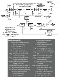
Figure 1 shows the time domain block diagram for a step response model. The normal operating value of the percent composition estimator input variable (%AVo ) is subtracted from the new value of the percent composition estimator input variable (value of the percent composition estimator input variable (%AVn) to create a percent analysis deviation variable (∆%AV) at point 1 that is added to the change in the disturbance value (∆%DV) to get the percent change in the estimator input with the disturbance correction as a process input (∆%XV) at point 2. The step response output is the normal operating value of the percent process variable (%PVo) added to a deviation variable (∆%PV ) that is the output of the series of dynamics blocks. The result is passed through a scaler block to provide a new value of the process variable (PVn) in engineering units at point 5. The dynamics inserted after the open-loop, steady-state process gain are a dead time block for the total loop dead time (θo) and a filter block for the secondary time constant (τs ) to provide all of the parameters for a second-order plus dead time step-response model.
The sign of the feedback signal added at point 4 in the estimator determines the type of open-loop process response. A negative value indicates negative feedback and hence a self regulating process. A positive value indicates positive feedback, a runaway process.
For integrating and runaway process models, the normal operating point of the manipulated variable that is the negative bias must be sufficiently greater than zero (e.g., 50%) to provide negative as well as positive changes in the process variable. This bias represents a process load. To achieve a new target or setpoint, the manipulated variable must be temporarily changed to be different from the load. The open-loop gain must also be large (e.g., > 2) to provide a full range of process variable response. When the process variable settles out at the new operating point, the manipulated variable returns to be equal to the load plus any compensation for the change in disturbance variable.The future value for an integrating process is the disturbance corrected composition estimator input value (∆%XV) multiplied by the open loop gain and a time interval for prediction (∆tf ) to give a change in the percent future value (∆%PVf) at point 6. This change is added to the normal operating point and passed through a scaler block to provide a future value of the process variable (PVf) in engineering units.
For synchronization with an at-line or off-line analyzer, the new value must be passed through a dead time block that is the analyzer dead time (e.g., sample transportation delay plus cycle time plus ½ analysis time). This new value of the process variable in engineering units that include the dynamics of the step response model and analyzer is compared to the actual measurement (e.g., at-line analyzer result). The new value for the step response model output subtracted from the actual measurement is the error in the prediction. The error is multiplied by a factor less than one (e.g., Kx = 0.4). The resulting fraction of the error is added to the future value in engineering units (PVf x) to provide a corrected future value (PVf) that is not slowed down by the process or analyzer dynamics. A PID loop or MPC can use the corrected future value as the controlled variable to provide incredibly fast control.
Rein in Runaways
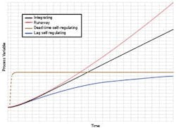
The block diagram (Figure 1) provides insight as to how the model changes depending upon the sign of process feedback within the process. The sign of the feedback signal added at point 4 in the estimator determines the type of open-loop process response (response with the PID in manual). A negative value indicates negative feedback and hence a self-regulating process. The open-loop response will settle out at a steady state for a given disturbance or PID output change. A zero value indicates zero feedback corresponding to an integrating process. The open-loop response will ramp until a physical or signal limit is reached.
The open-loop response of a dead-time-dominant process (a self-regulating process with a time constant much less than the dead time) is much different from self-regulating, integrating and runaway processes, and as a result the tuning rules are quite different.
A positive value indicates positive feedback, indicative of a runaway process (open-loop unstable process). The open-loop response will eventually accelerate, possibly to a point of no return. Open-loop tests on runaway processes are not done at all or long enough to show significant acceleration. These processes are designed to have large positive feedback time constants to slow down the acceleration. The process gain and positive feedback time constant of runaway is not identified by software but can be estimated based on ordinary differential equations (ODE).The online document "First Principle Process Relationships" shows how the process gains, time constants and dead times can be derived from ODE for all types of process feedback.
Figure 2 shows the open-loop response of self-regulating, integrating and runaway processes with an additional process classified as dead-time-dominant, which is a self-regulating process with a time constant much less than the dead time. While dead-time- dominant processes are not often seen due to thermal lags, the tuning rules are quite different. The online white paper "So Many Tuning Rules, So Little Time"details how tuning rules change with the type of process response.


