Engineering ranks efficiency and practicality over scientific or mathematical perfection in calculations, especially when the idealized mathematical perfection doesn’t match how nature behaves. However, sensibility with terms and equations often leads others astray, when the situation isn’t the same as the one that justifies shortcuts. Engineers more grounded in mathematical perfection might call those sensibilities downright sloppy.
Part one of this series examined confusing differences in engineering terms and calculations. Part two discusses the substitution of frequency for probability and omission of terms in propagation of probability.
Probability
Probability is the proportion (ratio) of the number of occurrences of an event in each number of trials that could generate the event, such as a theoretically expected proportion. For example, the probability of rolling a “four” on a standard, six-sided die is 1/6 = 0.16666, which would be stated as p (a four on one dice roll) = 0.16666. This is a theoretical value based on each side of the die having the same chance of showing on top. If you roll the die 6 million times, you expect to get the event of rolling a four to happen 1 million times. Then p = 1,000,000/6,000,000 = 0.16666.
This is the ideal true value, but only if the roll is randomized and the equal likelihood expectation of any number on top is true. Slight variation on the die dimensions or where the four is positioned when initiating the roll can make one number more favorable. The theoretical probability is an imagined reality, so it’s an estimate for reality.
However, even if all idealizations are true, you shouldn’t expect to get exactly 1/6 of the outcomes to be a four. Consider 10 rolls: 1/6 of 10 is 1.6666, and you can’t get 2/3 of an event. The outcome is either an event or not an event. Consider 600 rolls: you expect a four to emerge 100 times, but don’t be surprised if the random aspect of the trials ends with 98 times or 103 times. Nature won’t always provide the expected number.
There might not be a conceptual basis to theoretically determine the probability. In this case, you can observe past data (trials). For example, roll the die 100 times, and count the number of times a four comes up. Maybe it is 13 or 18. The estimate of the probability from past data will be 0.13 or 0.18, but this empirical value isn’t the true probability value. It’s an estimate from a limited number of trials. Although useful, neither method to determine probability returns an exact true value.
A trial (such as a die roll) can’t be cut in half. A trial is a completed batch of procedures. Pick up the die, shake it to randomize its orientation, toss it to roll on the table, and when it comes to rest, observe the number. You can’t derive an event outcome from half a roll because such scaling impossibility leads to alternate ways to analyze probability.
Frequency
Engineers often use the term “probability” to quantify the number of events that might (or did) happen in a time or space interval, but this is a frequency, or a rate, not a probability. For example, if the expectation is two events in one year, the frequency is two events per year, not the probability. One reason is probability must be between 0 and 1, inclusive.
An engineer might choose to reduce the time interval to three months, and say the expectation is 0.5 events per quarter. The resulting probability is 0.5, which is a legitimate value. However, it’s not advisable because, based on a one-week time interval, the rate is 2/52 = 0.03846. If probability is frequency, one choice makes the probability two, another 0.5, and another 0.03846. If the year is considered the trial, it can be halved; but with probability, you can’t have half of a trial. Again, events per year is not a probability. One clue that frequency is not probability is that you can divide the trial period to half a trial period.
Ideally, the Poisson distribution model converts the expected frequency of events (number of events per year, or per length, or per area) to the probability of events within that interval. The minimum number is zero, but there is no upper bound on the possible number of events. The idealization in the Poisson distribution model is that any event is wholly independent of any other event.
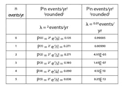
Use the expected or average rate or frequency (two per year, in this case) as lambda, λ, in a Poisson distribution model. In the equation, P(x)=(λn e-λ)/n!, n is the number of possible events in the time interval, and P(n) is the probability of that number of events. For example, if the expected rate is λ=two events/yr, then the probability of zero, one, two or three events is in Table 1.
There’s not only a probability of zero events in a year, but also 2, 3, 4, 5 or more events per year.
The expectation of two events per year doesn’t mean you’ll experience two events in any one year. You might not have any events, and the probability of no events in a year is 0.135. You might have four events, and the probability of four events in one year is 0.090. The probability of one event in a year is 0.271, which isn’t equal to the average frequency of two events per year.
If the expected frequency is very small, for instance if λ=1 event in 100 years=0.01/year, then the probability of two or more events in a year is vanishingly small, and the probability of one event in a year is P(1)=(0.011 e-0.01)/1!=0.099≅0.01=λ (Table 1). If frequency is small, it can approximate the probability.
Since the frequency and probability estimated from past and other processes, under different management conditions, are only estimates, and since the assumption that events are truly independent (no common cause), the error on equating probability to frequency is justifiable (when frequency is small). This convenience introduces an error, but the error is negligible relative to the uncertainty of the given data and the idealization in the model, so there’s no need to use perfect analysis.
If the expectation of the number of events scales with the duration of time or magnitude of the area (if you double the time, or double the area, you expect twice as many events), then use the Poisson distribution model.
Multiple trials
The expectation is that, after four coin flips (four independent trials), two will be “heads” because the probability of getting heads in any one flip is 0.5. However, there might not be any heads in the four trials, or one, two, three or four times in the set of flips.
The expected number of events scales with the number of independent trials. However, the number of possible events can’t exceed the number of trials because the limit contrasts with the unlimited number of possible events that characterizes a Poisson distribution model. The multiple independent trials and limit on the possible number of events are a clue to use the binomial distribution.
The binomial distribution is:
P(n|N)=(N!/(N-n)!n!)pnqN-n
P(n|N) means the probability of n number of events in N trials; p is the probability of an event in one trial; q=1-p is the probability of no event. The model idealization is that the events are wholly independent.
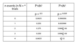
Ideally, the binomial distribution provides the probability of n number of events in N number of trials. For the coin flips, the probability of an event (heads) in a trial (a flip) is 0.5. For any of five possible outcomes, Table 2 indicates the ideal probability.
In the limit of low probability, such as a 0.001 chance of having an event in one trial, the probability of one event in four trials is about 0.003988≅0.004=4*0.001=4*p . Very small event probabilities mean the probability of an event scales with the number of trials. However, it’s not a mathematical truth.
The ‘and’ conjunction
Logical “and” conjunctions and reliability gates multiply the individual event probabilities. Ideally, if the probabilities of events A and B are independent of each other.
P(A AND B)=P(A)∙P(B)
For example, the probability of rolling a “three” on one die (p = 1/6) and flipping heads on a coin (p = 1/2) is 1/6*1/2 = 1/12 = 0.08333. In context of a process reliability analysis, if frequency is substituted for probability (because it’s a small value), and there are two full-sized pumps in parallel, the process stops if both fail. If the probability of one failing is 0.02 per year, if there are no common cause relations, and if it takes a month to repair/replace a failed pump, then the probability of both failing at the same time in a year is 0.02*0.02/12 = 0.00003333.
The ‘or’ conjunction
Logical “or” conjunctions and reliability gates are a bit more complicated. One way to obtain the “or” rule is to use the equivalent “not” condition. P(NOT A)=1-P(A). Then P(A OR B)=1- P(NOT (A OR B))=1- P(NOT A AND NOT B)=1-(1-P(A))(1-P(B))=P(A)+P(B)-P(A)P(B). So,
P(A OR B)=P(A)+P(B)-P(A)P(B)
For example, the probability of rolling a “three” on one die (p = 1/6) or flipping heads on a coin (p = 1/2) is 1/6 + ½ -1/6* ½ = 1/12 = 0.58333.
If the individual probabilities are small, then the product P(A)P(B) will be vanishingly small, and its impact can be ignored. Also, consider the individual P(A) and P(B) values aren’t known with certainty, and the complete independence of events A and B may not be true. The uncertainty of the givens and model idealization may be much larger than the contribution of discarding P(A) P(B). Conventionally, in reliability and safety analysis (with small frequency values substituted for probability), the “or” conjunction rule is shortened to:
P(A OR B)≅P(A)+P(B)
Know the differences
Keep aware of the difference between probability and frequency, and the independence idealization in the calculations. You can’t have half a trial. If the statement of probability permits cutting the trial period or area in half, it’s frequency, not probability. Only use the truncated “or” model when frequency or probabilities are low.


