It is proven that intensive, well-organized use of advanced process control (APC) can substantially increase the profitability of a plant. One of the key effects is reducing the ever-present variations in the process more than standard controllers or the operators can do.
This article explores how reducing the variance can lead to real, measurable credits, and describes the fundamental mechanisms. These mechanisms do, however, depend on the situation, so we need to first take a look at the three fundamental control scenarios:
- A process variable has to be kept closely at a given target value. This is the domain of regulatory control.
- There is no exact target figure given but only a direction. The variable in question shall be moved in this direction until a limitation is encountered. This is the domain of constraint control.
- Positive and negative influences exist on a certain general objective and we must find the optimal operating point, that is, the point where these positive and negative influences just balance out. This is the domain of optimization.
Because it is the most widely found scenario, we will focus on regulatory control where, for a certain process variable, a target value has been given that is considered to be the optimal value. The objective is to keep the variable closely at the target despite the influences that drive it away.
Case 1: No Limitations
How can we gain an economic advantage just by reducing variations of a target variable? Again, there are several different situations and mechanisms that we must consider separately to find the answer. We can only look at some of them here.
The first situation is where there are no limitations: The variable is not constrained by any limits that may come, for example, from the equipment or the product. In this case we need to consider the behavior of both the controlled variable and the variable we are using to steer the process (the manipulated variable). We distinguish between direct benefits, which relate to the controlled variable itself, and indirect benefits, which relate to the manipulated variable.
Figure 1: No Boundaries
In the case where there are no limitations, better control reduces the sum of deviations from the setpoint (shaded) and variations in the manipulated variable as indicated by the controller output OP.
Since the setpoint represents the optimal operating point for this variable, it follows that every deviation from this value represents an economic loss (Figure 1). This also means the loss is the greater the larger the deviation is and the longer it lasts. If we react too late or too weakly, the variable will move far away from the setpoint and return after a long time. Better and faster interaction will clearly reduce the excursions and shorten the time needed to return to the setpoint, resulting in the direct benefit of reduced economic loss.
Indirect benefits may come from integrated units, for example, using a stream from one unit as a heat source for another. In this case, any action in the first unit has an effect in the second one: a corrective action at one place causes a disturbance at another. Obviously, the smoother we act on the first unit, the smaller the negative effect on the other one will be. And the faster and the more precisely we act, the smaller the actions needed to resolve the situation and the lower the unwanted side effects.
Case 2: Closer to the Limit
The situation where there are limitations on the controlled variable is relatively common. A typical example would be where the feed stream to a reactor is heated in a furnace. The higher the temperature, the better the reaction, so we try to maximize the furnace coil outlet temperature (COT). However, the maximum allowable temperature may be limited by the tube material.
In this case, the setpoint of the COT controller must be a safe distance from that limit. The smaller the actual variations of the temperature, the smaller this safety margin can be. Through better control we can therefore move closer to the limit and gain the benefits (higher product yield or quality) from the higher reactor temperature.
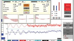
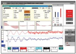
How close we can get to the limit can be calculated using several methods, including software developed for the purpose (Figure 2).
Case 3: Limits on Manipulation
In some situations there are limitations on the manipulated variable. A typical example is a batch reactor where the product should be brought to a certain temperature as fast as possible. We need to use the maximum heating or cooling capacity. However, examining the actual movements of the valves in the heating and cooling medium, we often see that they move quite extensively, sometimes as even 50-100%. Thus, on average, only 75% of the capacity is used.
Making the controller action smoother and reducing the movement of the valve from 50% to, for example, 20% would allow them to run on average at 90% opening. This can reduce the time to reach the new temperature, shortening cycles and resulting in increased unit capacity.
Case 4: Off the Line
Our last situations involve nonlinear effects. For example, we may have two variables (M and C) that have a linear relationship. Variable M, which is called the independent variable, has a certain effect on variable C, which is therefore the dependent variable. Any change in M will cause a change in C.
A dependent variable might be a product quality that is mainly influenced by a temperature. Examples of this situation can be found with distillation towers, where the impurity of the product streams is a function of the cutpoint and the fractionation, which in turn are indicated by suitable tower temperatures. Other examples are found with plug-flow reactors where the product conversion and quality are very much influenced by the product temperature at the reactor inlet.
If the relationship between the independent variable (the temperature) and the dependent variable (the product quality) was linear, it would not make any difference if we ran the temperature absolutely constant or if we ran it, for example, 10º above target for one hour, then 10º below target for an hour. The change in temperature causes exactly the same change in quality, no matter if the temperature is raised or dropped. The result: The average product quality is the same in both cases, as long as the average value of the temperature in the second case is the same as in the first case.
We could therefore state that in this (linear) case the average value of the dependent variable, here the product quality, is only a function of the average value of the dependent variable, here the temperature.
But in many processes, nonlinear relationships between variables are much more common than linear ones. This is also true for the examples given: The effects of the tower temperatures on the product qualities are nonlinear, as is the effect of the product temperature at the reactor inlet on conversion and qualities.
Figure 2: How High?
When a process variable is limited, improvement in the controller performance (here a reduction of the standard deviation by 50%) allows a significant step of the process variable (blue curve) toward the limit (light blue line).
The consequence of the nonlinear relationship is an increase in temperature will lead to a different change in the quality than a decrease. Running the temperature 10º above target for one hour, then for one hour 10º below target and so on would not give the same average quality. In fact, the average product quality would be worse. So we have to either tolerate the lower quality, which could exclude our product from certain applications, or compensate it, either by running at higher average temperatures (and thus higher cost) or by blending in some other higher-quality (and therefore higher value) material.
In the nonlinear case, the average value of the dependent variable is not only dependent on the average value but also on the magnitude of the variations of the independent variable. Reducing the variance of the independent variable will allow us to run closer to the ideal linear case and lower our extra costs and losses.
Squeeze and Shift
These examples show that significant improvements can be realized by improved control. One of the key basic mechanisms is reducing the variance of the variables, which subsequently allows us to move or shift the means of the variables. This is also called the double-S approach: Squeeze the variance and shift the mean.
The first important step for capturing these benefits of improved control is recognizing improvement opportunities. This requires that we monitor the dynamic performance of the key variables, and not just their average values, using a performance monitoring system. Once the current performance of the process variables is known, we can estimate the potential shift in a mean value made possible by variance reduction. We can then calculate the final effect of a change on product yield or quality, and thus the economic benefits.
These actions take a certain effort, but the first step, the monitoring of the dynamic behavior, requires very little. Wherever these methods have been applied in a consequent way, the results have brought back the investment many times.
The achievable credits from reduced variance depend on the situation, of course, but improvements of 5% in product qualities and yield or utility consumption are common, and even 10% are not infrequent. In one extreme case, reported increase in the capacity of an aluminum rolling mill was 170%.
Hans Heinz Eder, president of optimization and control consulting company ACT, worked for more than 20 years as process designer, advanced control engineer, APC manager, training coordinator, and CIM advisor with Exxon. He may be reached at [email protected].
Latest from Home

Leaders relevant to this article:


