A chemical plant may have thousands of measurements and control loops. By the term "plant-wide control," I do not mean the tuning and behavior of each of these loops, but rather the control philosophy of the overall plant with emphasis on the structural decisions:
- Selection of controlled variables (CVs, "outputs")
- Selection of manipulated variables (MVs, "inputs")
- Selection of (extra) measurements
- Selection of control configuration (structure of overall controller that interconnects the controlled, manipulated and measured variables)
- Selection of controller type (PID, decoupler, MPC, linear, quadratic, Gaussian (LQG), aka, optimal control, ratio, etc.).
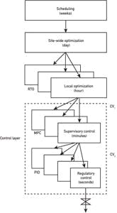
In practice, the control system is usually divided into several layers, separated by the time scale (Figure 1).
Figure 1. Typical control hierarchy in a chemical plant.
Control structure design (plant-wide control) thus involves all the decisions necessary to make a block diagram or process and instrumentation diagram that includes the control system for the entire plant, but does not involve the actual design of each individual controller block.In any mathematical sense, the plant-wide control problem is a formidable and almost hopeless combinatorial problem, involving a large number of discrete decision variables. In addition, the problem is poorly defined in terms of its objective. Usually in control, the objective is that the CV (output) should remain close to its setpoint.
However, what should we control? The answer lies in considering the overall plant objective, which is to minimize cost, that is, maximize profit, while satisfying operational constraints imposed by the equipment, marked demands, product quality, safety, environment and so on.
Actually, the "original" mathematical problem is not so difficult to formulate, and with today’s computing power, it may even be solvable. It would involve obtaining a detailed dynamic and steady-state model of the complete plant; defining all the operational constraints; defining all available measurements and manipulations; defining all expected disturbances; defining expected, allowed or desirable ranges for all variables; and then designing a nonlinear controller that satisfies all the constraints and objectives, while using the possible remaining degrees of freedom to minimize the cost. This would involve a single centralized controller that, at each time step, collects all the information and computes the optimal changes in the manipulated variables.
Although such a single, centralized solution is foreseeable on some very simple processes, it seems to be safe to assume that it will never be applied to any normal-sized chemical plant. There are many reasons for this, but one important one is that, in most cases, one can achieve acceptable control with simple structures, where each controller block only involves a few variables, and such control systems can be designed and tuned with much less effort, especially when it comes to the modeling and tuning effort. After all, most plants operate well with simple control structures.
Real-World Control
So how are real systems controlled in practice? The main simplification is to deconstruct the overall control problem into many simple control problems. This deconstruction involves two main principles:
- Decentralized (local) control. This "horizontal deconstruction" of the control layer is mainly based on separation in space, for example, by using local control of individual process units.
- Hierarchical control. This "vertical deconstruction" is mainly based on time scale separation (Figure 1).
We generally have more centralization as we move upwards in the hierarchy. Such a hierarchical (cascade) deconstruction with layers operating on different time scales is used in the control of all complex systems.
The upper three layers in Figure 1 deal explicitly with economic optimization, and are not considered here. We are concerned with the two lower control layers, where the main objective is to track the setpoints specified by the upper layers. A very important structural decision, probably more important than the controller design itself, is the choice of controlled variables (CVs) that interconnect the layers. More precisely, the decisions made by each layer (boxes in Figure 1) are sent as setpoints for the CVs to the layer below.
A Plant-Wide Control Procedure
No matter what procedure we choose to use, the following decisions must be made when designing a plant-wide control strategy:
Decision 1—Select "economic" (primary) controlled variables (CV1) for the supervisory control layer (the setpoints CV1 link the optimization layer with the control layers);
Decision 2—Select "stabilizing" (secondary) controlled variables (CV2) for the regulatory control layer (the setpoints CV2 link the two control layers);
Decision 3—Locate the throughput manipulator (TPM);
Decision 4—Select pairings for the stabilizing layer, that is, pair inputs (valves) and controlled variables (CV2). By "valves," I mean original dynamic manipulated variables.
The key idea is to start top-down with the economics and identify the various operating regions (Figure 1). In each of these regions, we need to identify the controlled variables that link optimization and control. After an intermediate step where we consider the location of the throughput manipulator, we proceed with the bottom-updesign of the stabilizing layer. The goal is to find a simple control structure that combines all the possibly conflicting objectives with minimal need for switching and other kinds of supervisory control.
Overview of Plant-Wide Control Procedure—Top Down
Top-down analysis (focus on steady-state economics) begins with Step 1—Define operational objectives (economic cost J to be minimized) and constraints. A systematic approach to plant-wide control requires that we first quantify the operational objectives with a scalar cost function J (or equivalently, a scalar profit function, P = -J). This is usually not very difficult, and typically we have J = cost feed + cost utilities (energy) – value products.
The goal of operation (and of control) is to minimize the cost J (or equivalently, to maximize the profit P = - J). The cost J should be minimized subject to satisfying the operational constraints, including safety and environmental constraints.
Typical operational constraints are minimum and maximum values on flows, pressures, temperatures and compositions. For example, we always have that all flows, pressures and compositions must be non-negative.
Step 2—Identify degrees of freedom (MVs) and optimize the operation for important disturbances (offline analysis) to identify regions of active constraints. Identifying the economic (usually steady-state) degrees of freedom is not usually as simple as one would expect. One approach is to first identify all the (dynamic and steady-state) control degrees of freedom (inputs, "valves"), and then subtract the ones with no steady-state effect. The optimization of the plant for expected operation is usually the most time- consuming step. Note that there are two main modes of operation Mode I. Given throughput. Maximize efficiency.
Mode II. Throughput is a degree of freedom. Find optimal throughput (often this equals maximum throughput). Maximize throughput (with production rate as a degree of freedom).
Although the plant and its control system are most often designed for Mode 1, usually the most profit is made when product processes are high and optimal operation is the same as maximum throughput (Mode II). Plant-wide control should generally be focused much more on Mode II.
Step 3—Selection of primary controlled variables (CV1) (Decision 1). "What should we control?" This question has been the main topic for my research in the plant-wide control area over the last 25 years, and I think I finally have found the solution:
- Control active constraints
- Control "self-optimizing" CV1s for the remaining unconstrained degrees of freedom.
In particular, the research has been focused towards the latter unconstrained CV1s. "Self-optimizing" means that when the selected variables are kept constant at their setpoints, then the operation remains close to its economic optimal in spite of the presence of disturbances.
In general, the controlled variables (CV1) will be individual measurements or combinations of measurements. Thus we can write, CV1 = H y. Here, y contains all the available measurements (including MVs) and H is the selection or combination matrix to be found. [See V. Alstad, S. Skogestad and E.S. Hori, "Optimal Measurement Combinations as Controlled Variables," J. Proc. Control, 19, 138-148, 2009.]
Step 4—Select location of throughput manipulator (TPM) (Decision 3).
The main purpose of a process plant is to transform feedstocks into more valuable products, and this involves moving mass through the plant. The amount of mass moved through the plant, as expressed by the feed rate or product rate, is determined by specifying one degree of freedom, which we call the TPM.
In addition, most plants have one TPM, but complex plants with six parallel units and multiple or alternative products may have more. From a steady-state point of view, the location of the TPM does not matter, but it is important dynamically.
There are two main concerns when placing the TPM:
- Economics—This is relevant when the plant is operated at maximum capacity. The TPM should then be located close to the bottleneck to reduce the back-off from the active constraint that has the largest effect on the production rate.
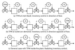
- Structure of the regulatory control system—Because of the radiation rule, the location of the throughput manipulator has a profound influence on the regulatory control structure of the entire plant (Figure 2).
Figure 2. Radiation rule: Need radiating inventory control around a fixed flow (TPM). From, Price, R. M., & Georgakis, C. (1993). "Plant-Wide Regulatory Control Design Procedure Using a Tiered Framework." Industrial and Engineering Chemistry Research, 32, 2693–2705.
An underlying assumption for the radiation rule is that we want "local consistency" of the inventory control system. [See E.M.B. Aske and S. Skogestad, "Consistent Inventory
Control," Ind. Eng. Chem. Res, 48 (44), 10892-10902, 2009.] This means that the inventory in each unit is controlled
locally, that is, by its own inflows or outflows.
In theory, one may not require local consistency, and allow for "long" inventory loops, but this is almost never done for obvious operational reasons, including risk of emptying or overfilling tanks, start-up and tuning and increased complexity.
Plant-Wide Control Overview–Bottom Up
Bottom-up analysis (focus on dynamics) begins with Step 5—Choose structure of regulatory (stabilizing) layer. The purpose of the regulatory layer is to stabilize the plant, preferably using a simple control structure with single-loop PID controllers. "Stabilize" here means the process doesm’t drift away from acceptable operating conditions when there are disturbances. Also, the regulatory layer should follow the setpoints given by the "supervisory layer."
Reassignments (logic) in the regulatory layer should be avoided. Preferably, the regulatory layer should be independent of the economic control objectives (regions of steady-state active constraints), which may change, depending on disturbances, prices and marked conditions. The main decisions are:
- Identify stabilizing CV2s. These are typically drifting variables, such as levels, pressures, reactor temperature or the temperature profile in distillation column. In addition, active constraints (CV1) that require tight control (small back-off) may be assigned to the regulatory layer. This usually isn’t necessary with tight control of unconstrained CVs because optimum is usually relatively flat. Also, note that we do not "use up" any degrees of freedom in the regulatory control layer because the setpoints CV2 are left as manipulated variables (MVs) for the supervisory layer. To some extent the choices for CV1 and CV2 (Decision 1) are independent of each other.
- Identify pairings (MVs to be used to control CV2 (Decision 4)), taking into account the following:
- Ensure "local consistency." You want local consistency for the inventory control [Aske and Skogestad, 2009]. This implies that the inventory control system is radiating around the given flow.
- Control constraints. You want tight control of important active constraints (to avoid back-off). The main rule is to "pair close."
- Avoid selecting as MVs, in the regulatory layer, variables that may optimally saturate (steady-state), because this would require either reassignment of regulatory loop (complication penalty) or back-off for the MV variable (economic penalty).
Step 6—Select structure of supervisory control layer. Objectives of supervisory layer:
- Switch control structures (CV1) depending on operating region.
- Perform "advanced" economic/coordination control tasks:
- Control primary variables CV1 at setpoint using as degrees of freedom (MV): Setpoints to the regulatory layer (CV2s)
- "Unused" degrees of freedom (valves)
- Keep an eye on stabilizing layer
- Avoid saturation in stabilizing layer (which usually requires back-off and thus economic penalty)
- Feed-forward from disturbances (If helpful)
- Make use of extra inputs
- Make use of extra measurements
Step 7—Select structure of (or need for) optimization layer (RTO). Ask the question, is this even necessary? Do we need such a structure?
Implementation
Alternative 1—"Advanced single loop control" = PID control with possible "fixes," such as feed-forward (ratio), decouplers, logic, selectors and split-range control. (In many cases some of these tasks are moved down to the regulatory layer). With single-loop control an important decision is to select pairings. Note that the issue of finding the right pairings is more difficult for the supervisory layer because the interactions are usually much stronger at slower time scales.
Alternative 2—Multivariable control (usually MPC).
Conclusion
This article presents the current version of the systematic plant-wide control procedure. It’s still being updated and tested on applications, but after having worked on this issue of about 25 years, I have good hopes of converging at final procedure by about the year 2025.
[Editor’s note: An extended version of this article is at www.controlglobal.com/whitepapers/2011/004.html.]
Latest from Flow

Leaders relevant to this article:
