THE TIME it takes to bring a slow process variable from its minimum or maximum to set point is a significant portion of a batch or startup phase. The more important analytical loops, pressure, and temperature loops often have a response that ramps most of the way to set point.
In batch processes, the ramp is most likely due to the process actually having an integrating response because the discharge valve and possibly the vent valve are closed at the start of the batch. The outlet valves may also be closed in continuous processes when a vessel is being filled or pressurized.
Even when the startup of a continuous loop is delayed until after an outlet flow is established, the small dead time and large time constant of a well-mixed volume results in a loop response that looks like an integrator. Even more problematic is the runaway response, where the process variable actually starts to accelerate. All of these responses benefit from special considerations, such as using a Lambda factor of less than 1.0 and pre-positioning of valves, as discussed in “Life's a Batch,” CONTROL, June ’05, and in a dozen Control Talk columns on process control techniques and tuning for batch processes.
Most of the articles and books on tuning loops concentrate on set point and load changes around operating point. For integrating processes, the focus is on surge tank level loops because these are the major source of variability in a plant because they jerk feeds around or cause a rolling action primarily from too much reset action (too little reset time). Bringing a composition, pressure, or temperature rapidly from either end of the scale to a set point is a different story.
Nothing Says Forever Like Tradition
There are four major practices for starting up a loop with a large process time constant or slow ramp time compared to the dead time. These loop practices for fast batch and startup response are:
- Switch controller to auto with the final set point
- Switch controller to auto with an initial set point, and then switch to final set point
- Put controller in manual or output tracking with final set point, set valve to its normal position, wait, and switch to auto
- Put controller in manual or output tracking with final set point, set valve to extreme position, wait, switch valve to normal position, wait, and switch to auto
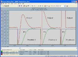
Figure 1 shows the batch or startup response of a pressure loop with an integrating response for practices 1, 2, and 4. Practice 3 isn’t shown because it’s not viable for integrating processes. There are other practices, such as ramping the set point, for unit operations, where it’s desirable that the approach of the process variable to set point and the output to its final resting value is moderated or that a profile be enforced.
FIGURE 1: BATCH AND STARTUPIn practices 1 and 2, the controller output is at its initial value at one end or the other of the output scale (often zero). All methods assume the pump and block valves have already been started and opened, respectively.
In Practice 1, if the loop is tuned to minimize variability in the controller output, which is the case for surge-volume level control, the batch phase may time out before the process reaches set point. For example, if the process time constant is 50 min, and a Lambda factor of 5 is used, then the closed-loop time constant is 250 minutes, and the time to reach 98% of set point is 1,000 min (or four closed-loop time constants). A similar situation exists for slow ramp rates. For integrating processes, the Lambda factor is the ratio of the closed-loop arrest time to the open-loop arrest time. The arrest time is the time it takes for a PV to make a designated allowable excursion for a given upset. If the response is a runaway, then vessel relief devices or interlocks might activate if the Lambda factor is greater than 1. The vessel could get off the ground before the loop gets off the ground.
A dead time much faster than the process time constant or ramp rate means that usually a Lambda factor of less than 1 (closed-loop time constant or arrest time less than the open-loop time constant or arrest time) is permissible for stability, and desirable for fast control of these process variables. This is particularly important for Practice 1 because you’re relying on reset action to get you to set point. All of the batch or startup responses in Figure 1 use a Lambda factor less than 1.
In Practice 2, the set point is changed from its initial to final value at one execution or more after the controller is switched to auto. Note that, if you switch the set point within the same execution of the module as the switch of the mode, then you’ll probably end up with the same response as Practice 1. In the second batch or startup response, the set point change kicks the output, which gives the process variable a boost on its way to set point. The time to reach set point (rise time) is nearly cut in half, but the settling time is about the same. Since, the overshoot is minimal, the rise time might be more important. Also, the controller tuning could be tweaked to reduce settling time.
Many astute automation engineers will preposition the controller output by what is called a “head start” or “process action.” For self-regulating loops, the valve position might set at what was considered to be a normal throttle position or final resting value (FRV) seen from previous trends when the process variable had settled out at set point. This corresponds to a Lambda factor of 1 because, if held at this position, it will drive the process variable with a time constant equal to the process time constant.
For integrating and runaway responses, the process variable won’t go anywhere until the valve is positioned beyond its FRV. This leads to Practice 4, in which the valve is set to an extreme position allowed by the process to give the fastest approach to set point. Next, the brakes are slammed on, so the process variable doesn’t run over the set point. It’s kind of like driving in Italy. The question is when do you hit those brakes?
The Wait
Short of having an Italian taxi driver operate your loop, what can be done to get the loop to its destination the fastest way possible?
The plot for Practice 4 shows the response for a technique briefly described in “Peak Concerns,” Control Talk, CONTROL, April ’05. The rate of change is computed from the change in the process variable (PV) over a time large enough to get a good signal-to-noise ratio. The old value of the PV, created by passing the PV through a dead time block, is subtracted from the new PV. The Δ PV is divided by the block dead time to create a rate of change. The rate of change multiplied by the process dead time is then the predicted change in the PV that, when added to the new PV, is the predicted end point shown in Equation 1. When the end point equals or exceeds the final set point, the controller output is switched from maximum throttle to its FRV. It’s held at this FRV for one process dead time, and is then released for feedback control. This method compensates for nonlinearities and disturbances that are evident when it’s time to hit the brakes.
EQUATION 1
PVf = [(PVn – PVo) / DT] * td + PVn
Where:
PVf = predicted PV one dead time into the future (%)
PVn = new PV (%)
PVo = old PV (output of dead time block) (%)
DT = DT block dead time (sec)
td= total loop dead time (sec)
If the process dead time is underestimated, the loop will overshoot the set point. Therefore, it’s important to be generous in the dead time estimate. It’s especially important the dead time not be too short for zero-load integrating process (as described in the “Peak Concerns” column), where the FRV is zero and there’s nothing to bring back the process variable to set point. Also, a safety margin should be added to the dead time estimate for runaway processes since the process is accelerating.
Without Dead Time I’d Be Jobless
If the loop dead time is zero, the loop could switch to the FRV when the PV reached set point. Furthermore, the sky’s the limit for the controller gain, and feedback action could provide instantaneous correction. My lifestyle is largely the result of dead time. A better term than process dead time is “total-loop dead time” because there are many sources of dead time outside the process.
The biggest source of slow ramp times and process time constants is measurement and valve resolution. The time it takes for the change to get through the resolution limit is dead time. Dead time from the measurement and valve resolution are inversely proportional to the rate of change of the process variable and controller output, respectively. Consequently, for closed-loop tests, identified dead time depends on the controller tuning and size of the set point’s change. Fortunately, changes in valve position are quite large, and dead time from resolution is minimal for the optimal switching method described in Practice 4.
Other sources of instrument dead time include measurement transportation delay, sensor lags, transmitter dampening, analog and digital filters, module execution time, valve dead band, and actuator pre-stroke dead time.
An adaptive controller can identify the total-loop dead time accurately, if the trigger point, in terms of output changes, are large enough. Note that the ultimate proof of the pudding is the output change, rather than the set point change, because it includes the effect of tuning, and is ultimately what’s driving the process. Given the measurement and valve resolution, the adaptive controller, with its knowledge of the integrating process gain, can correct the observed dead time to give a value closer to the output changes associated with the optimal switching. For a 12-bit A/D and 1 sign bit, the measurement resolution is 1 in 11 bits, or about 0.05% of span. Consequently, large temperature spans from using multiplexed I/O instead of dedicated transmitters are a major source of dead time in reactor temperature loops. The valve resolution can vary from 0.1% for a sliding stem valve with a digital positioner to 10% for a ball valve with high friction packing and no positioner. Since valve resolution caused many failures of adaptive controllers, newer technologies identify the valve resolution online. A digital positioner can give a position reading back to the control system to make this identification much faster.
An adaptive controller also can identify the integrating process gain. This can be used with the current ramp rate and the pre-positioned extreme controller output to estimate the FRV in Equation 2. Note that, if the extreme output (OUTx) is less than the FRV, the signs of each expression are reversed to get a positive FRV. Of course, limits should be enforced on the calculated value and it may be desirable to use a portion of the difference between the calculated FRV and the last captured FRV added to the last captured FRV to estimate the new FRV. For primary loops in a cascade control system, the extreme output must match up with the set point limits of the secondary loop and the FRV is a set point of the secondary loop. It’s necessary to keep the units of the process variable and output and the process integrating gain consistent. If process integrating gain is in %/sec/%, the process variable and output must both be in %. For integrating processes and OUTx > FRV:
EQUATION 2
FRV = OUTx – [(PVn – PVo) / DT] / Ki
Where:
FRV = final resting value (%)
Ki = integrating process gain (%/sec/%)
OUTx = output at extreme allowed by process (%)
PVn = new PV (%)
PVo = old PV (output of dead time block) (%)
DT = DT block dead time (sec)
With a little ingenuity, similar equations can be developed for estimating the FRV of self-regulating and runaway processes based on an identified process gain. These equations can be put online in the observation mode to see how well they estimate the FRV before it’s actually used for Practice 4. If the FRV is too variable and can’t be accurately captured or calculated, it’s best to revert back to Practice 2. Practice 2 depends more heavily on the controller’s tuning and in particular on the relative amount of proportional and reset action because the tuning is responsible, not just for correcting the FRV, but for taking the output all the way from its extreme to the FRV. It’s important that gain dominates reset action in the approach to set point. Proportional action must kick the output to the allowable extreme, and then back it off as the PV approaches set point, despite the effect of reset action, which works to force the output to its limit until the PV crosses set point.
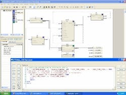
FIGURE 2: OPTIMAL SWITCHINGNext Destination
The optimal switching technique based on rate of change of the PV is ideally suited for an integrating or ramping process, but works well for self-regulating and runaway processes, where the fastest possible approach to set point is desired. For runaway processes, the dead time used for prediction should be increased since the PV is accelerating. These and other process control techniques can save 25% or more in batch cycle and startup time. Generosity in the dead time estimate is rewarded by helping you get to your next destination, which just might be happy hour.
| About the Author |


