Model-based control: Raspberry Pi vs programmable logic controllers

[For a video presentation of this article, visit
https://www.youtube.com/watch?v=0eZdNMJDlJU&feature=youtu.be]

In 2017, Control’s sister publication, Control Design, published an article demonstrating how an Arduino single-board microcontroller for do-it-yourself applications could control a flow loop when integrated with industrial-grade instruments and control devices. It compared this inexpensive “maker” approach to using a simple and commercially available industrial programmable logic controller (PLC) configured to carry out the identical task.

The widespread interest generated suggested a follow-up investigation using more complex controllers for more demanding processes. The new challenge: performing model-based control with two input variables using a Raspberry Pi, compared to performing the same task with a basic PLC.

System block diagram

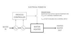
Figure 1: The process controller acts entirely on the process model and does not have a measurement of T_OUT available. Based on F_IN and T_IN, the program determines how much heat needs to be added.

The process in this case is a small hot-water heater. The objective is to control the output temperature, not with a PID loop or high/low thermostat-like control, but by measuring the inlet water temperature and flow rate, and calculating the amount of added heat necessary to reach the outlet temperature setpoint. This approach provides a more immediate process adjustment for two variable inputs and should keep the temperature more stable than a conventional loop. The test setup represents any process where two independent and unrelated inputs, in this case flow and inlet temperature, affect output in a predictable way allowing the process model to respond to both.

Creating the process model

Creating a process model requires detailed quantitative understanding how these factors affect the outlet temperature: water flows in, energy is applied to the heating element and warmer water flows out. The goal is to maintain a desired water temperature at the outlet under all conditions (Figure 1). All process parameters (Figure 2) work together to determine one thing: how much to run the heater to achieve the desired output temperature. (For more detailed discussion of the process model, including the control equations, see the following appendix.)

Process model parameters

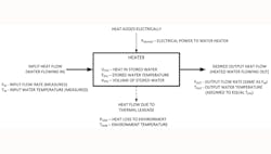
Figure 2: The model depends on a critical quantitative understanding of all the variable and constant characteristics of the process.

To make the project more challenging and ensure there is no cheating, the outlet temperature is measured but not fed to the controller. It appears simply on a display to verify the reading.

Implementing the control strategy

This project’s objective is to perform the same functions on two different platforms: a standard industrial PLC using ladder-logic programming, and a Raspberry Pi 3 Model B programmed in Python under the Raspbian OS (based on Linux OS). Both hardware platforms use the same sensors and control interfaces (Figure 3).

Controller block diagram

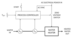
Figure 3: Both controllers use the same sensors (RTD and flow meter) and actuator. They also both use the same model parameters so they should perform very similarly.

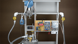
Figure 3a: Equipment with the Raspberry Pi controller. (Heater unplugged for clarity.)

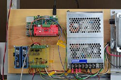
Figure 3b: Close-up of Raspberry Pi hardware setup.

Figure 3c: Equipment with the CLICK PLC controller. (Heater unplugged for clarity.)

The flow, F_IN, is measured by an Emerson Rosemount 3051SFP integral orifice differential pressure flow meter (Figure 4). It communicates via 4-20 mA current loop.

The temperature sensor T_IN uses a 100-ohm platinum resistance temperature detector (RTD), mounted at the inlet to the water heater (Figure 5).

A solid-state TRIAC relay with a zero-voltage switching interface controls ac power to the water heater, driven by a single-bit discrete output from the controller. The algorithm operates on a once per ac cycle basis, with timing sensed from the ac power line via a discrete input (Figure 6). The nature of the sensing circuit as implemented means the controller has about 4 milliseconds from the start of the pulse to run its calculations and decide whether to turn on the relay for the next full ac cycle.

Two operator controls are provided (Figure 7): a pushbutton discrete input for a start/reset function, T_TARGET, plus a potentiometer analog input for the temperature setpoint. Pressing the pushbutton causes the controller to start the control algorithm, and the operator can adjust the potentiometer to the desired T_TARGET.

Working with the hardware

The primary objective of this project is comparing design and implementation experiences between the two controller platforms. Let’s look at them individually.

The PLC implementation uses AutomationDirect’s CLICK PLC hardware (Figure 8):

C0-12DD1E-2-D; Ethernet Analog PLC
C0-04RTD; Temperature Input Module for the RTDs
C0-04AD-1; 4-20 mA Input Module for the flow meter
C0-01AC; 24 Vdc Power Supply

The PLC includes an Ethernet interface for programming, discrete inputs and outputs, and 0-10 V analog inputs. The flow meter and RTD connect directly to their respective modules.

The Raspberry Pi 3 Model B v1.2 is, for all practical purposes, a personal computer motherboard. It includes:

Quad Core 1.2 GHz Broadcom BCM2837 64-bit CPU with 1 Gb RAM
10/100 wired Ethernet RJ45
40-pin extended GPIO
Micro-SD port for loading the OS and storing data.

That’s quite a bit for a very low price, making it attractive for this type of project. On the other hand, the Raspberry Pi has few mechanisms to interface with industrial devices. It has a set of general-purpose I/O (GPIO) signals that can be programmed as inputs or outputs and which can be used to trigger interrupts. However, it lacks any native analog I/O capability.

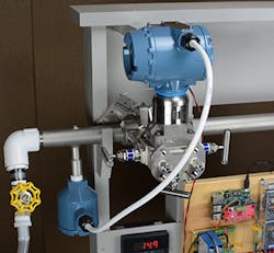
Figure 4: The Rosemount 3051SFP flow meter is set with an operating range from 0.5-2.0 gpm and sends its data to the controller via a conventional 4-20 mA current loop.

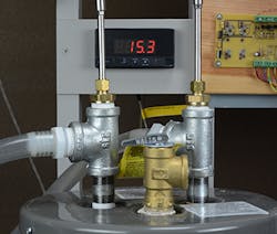
Figure 5: The hot water heater has two RTDs, monitoring the inlet and outlet temperatures (T_IN and T_OUT), right and left, respectively. T_IN is fed to the controller but T_OUT appears only on the display.

Fortunately, there are boards to plug onto the GPIO pins to provide this capability, including a Makerfabs ORS1115AD four-channel A/D module used here. This provides four 16-bit, 0-3.3 V analog inputs (no live zero) with a screw terminal strip to simplify wiring. We still need access to some GPIO pins to sense the power line, read the start pushbutton, and control the zero-voltage switch. A breakout board provides screw terminal access to the GPIO pins, while passing necessary signals up to the A/D module. This results in a stack of three boards (Figure 9) supported by the pins: Raspberry Pi 3 on the bottom, breakout board in the middle, and A/D module on top.

The pushbutton and control potentiometer interfaces are straightforward and connected directly. The zero-voltage switch is isolated, but requires more voltage than the 0-3.3 V Raspberry Pi GPIO pin. RTDs require external conditioning to produce a suitable signal for A/D inputs. Rather than design a signal-conditioning circuit from scratch, an old Analog Devices 5B34-01 RTD Input Module purchased at a hamfest flea market does the job. This device provides a 0-5 V output for a -100 to 100 ˚C temperature range. Given the 0-3.3 V environment, an op-amp circuit is required to provide necessary scaling. The current-loop input for the flow meter was simpler, as a 165 ohm resistor converts the current to a non-isolated voltage scaled for the 3.3 V analog input.

A small printed wiring board (PWB) was designed to handle all of this circuitry (Figure 10). The Raspberry Pi depends on all of the functions provided by this PWB, while the CLICK PLC only uses the power line sensing circuit and the zero-voltage switch circuit as a tie point.

Comparing Programming Approaches

The CLICK PLC and Raspberry Pi provide radically different programming environments. The PLC uses traditional ladder logic, while the Raspberry Pi allows a plethora of programming language possibilities, although Python is the out-of-the-box choice. CLICK PLC programming software runs on a Windows PC, providing a graphical interface for creating the ladder logic, downloading it to the PLC, and monitoring execution. For all the Raspberry Pi programming and operating we worked with a monitor, keyboard and mouse connected to the controller.

The CLICK PLC is programmed using ladder logic, where every action depends upon conditions. With every scan, the internal processor evaluates inputs and other internal state conditions, defining which actions to do. Thus, when a one-second timer completes, the flow and inlet temperature are read. Another contact representing the 60 Hz power line timing input coordinates the zero-voltage switch control. CLICK PLCs allow both the rising and falling edges of a signal to be used and are fast enough to recognize each ac cycle and operate the zero-voltage switch as needed.

60 Hertz power line timing sense

Figure 6: Both controllers use zero-voltage switching, which necessitated adding a circuit to sense the 60 Hz current in capacitor C1 so the controller can turn on the element at the appropriate time.

Raspberry Pi controllers are extremely flexible, but Python was programming was chosen for simplicity. Python is procedural, executing statements in top-to-bottom order. When started, it executes an initial function and can call other functions in response to external events. Three functions provide the initialization, one-second readings of inlet temperature and flow, and the 60 Hz heater control. Printing all the variables on the screen every second in one long line helps with debugging, however making a correction requires stopping the program, doing the edit, and then restarting it.

Comparing effectiveness

Both the Raspberry Pi and the CLICK PLC can run the program, drive the heater and maintain a specified outlet temperature.

The CLICK PLC controls the water heater in a very predictable way. Most of the time, the solid-state relay indicator light flickers on and off, but sometimes stays off or on briefly. These sustained instances are probably due to variations in reading the input parameters (flow and inlet temperature), where a reading changes slightly, and then changes back. All in all, the CLICK PLC is effective and stable.

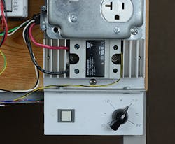
Figure 7: The potentiometer to adjust the setpoint and the start/reset pushbutton are mounted with the solid-state relay controlling the heating element.

Figure 8: The four CLICK PLC modules interlock and communicate through a system of internal pins.

The Raspberry Pi is also able to maintain the desired temperature, but the indicator light flickering is more irregular. Since both the CLICK PLC and the Raspberry Pi run the same algorithm, the differences are likely with the input interface to the flow meter and RTD. The Raspberry Pi’s 16-bit A/D converter may be more susceptible to low levels of signal noise.

Another concern with the Raspberry Pi is the 60 Hz interrupt code which uses variables created from the one-second loop. Since the 60 Hz interrupt is not synchronized with the one-second loop, it could interrupt anywhere in the one-second code, potentially even at a point where a variable is partially updated, causing the 60 Hz code to use an improper value.

Both the noise filtering issue and the timing issue could be resolved with more extensive programming efforts, which would be warranted for a production system.

Overall impressions

For simplicity and effectiveness, the CLICK PLC was the clear winner:

Straightforward programming
Consistent behavior
Ladder logic avoids critical regions with asynchronous execution

From a hardware perspective, the PLC natively supports RTD signal conditioning and 4-20 mA current loop instruments. The only interface needing external circuitry was the 60 Hz detection from the ac power line.

The Raspberry Pi software, using its native Python programming environment, took us barely a day to write and debug. But, since Python is procedural and this application is interrupt driven, it creates a layer of complexity to avoid timing problems. Also, the Raspberry Pi runs a variant of the Linux operating system, which must multi-task operations including the system I/O interfaces, monitor, keyboard, mouse, and more. This adds uncertainty for executing the faster near-real-time program tasks.

Finding all the I/O hardware needed for the Raspberry PI was a chore. The pass-through breakout board was available in the “maker” section of a local computer store, but an online search was needed to find the analog module, which had to be shipped from China. Since the analog module only senses 0-3.3 V, signal conditioning was required for both the RTD and flow meter, requiring us to design a custom printed wiring board.

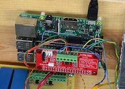
Figure 9: Creating the necessary infrastructure for adding I/O to the Raspberry Pi requires stacking multiple boards on the GPIO pins, which is a bit fragile.

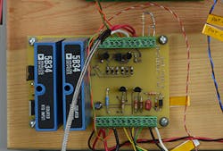
Figure 10: Adding circuitry for RTD and flow meter signal conditioning along with ac current sensing for the Raspberry Pi required an external board. Provision was made for a second RTD but it was not used.

As a practical matter, the Raspberry Pi, with its multi-tasking operating system, is not a good fit for this sort of real-time control. It could shine as an operator interface since it integrates monitor, keyboard and mouse with a file system on an SD card but it needs a great deal of effort to create industrial interfaces. With better interfaces and a more robust physical arrangement than stacking fragile boards, it would be more competitive.

A detailed cost analysis is not part of this investigation, but there are some general observations. From a standpoint of raw product costs, the PLC platform solution clearly costs more than the consumer electronics implementation. However, factoring in the additional engineering effort to create hardware interfaces and programming labor to replicate typical PLC functionality makes the Raspberry Pi less attractive. In addition, there is a question of how robust each solution is for industrial applications.

Industrial suitability

A user considering choosing one of these approaches for a serious industrial application has to ask, “Which do we want on our equipment?” With a PLC there is generally more automation-specific processing going on in the background than is evident when looking at the program. This enhanced functionality would need to be carefully added into a Raspberry Pi implementation.

PLCs include software watchdogs keeping an eye on the program to make sure it is executing as it should. For example, poor programming could lead to code execution in an endless loop, causing a harmful and potentially dangerous out-of-control situation. The software watchdog monitors the duration of each program scan. If a given scan is not completed in the allowable time, the dog will bark, fault the PLC and put it into a safe state while alerting the operator.

Hardware watchdogs keep an eye on the devices connected to the PLC, particularly I/O modules or individual devices such as switches, sensors and actuators. The PLC is always exchanging handshakes with the modules and evaluating analog under-range and over-range conditions. Depending on how the program is set up, any trouble may put the PLC into a safe state or at least inform operators of the problem.

All of these functions are designed to warn users if the PLC believes it is not functioning as expected and therefore cannot control the machine or process as desired. Furthermore, the industrial packaging of PLC components themselves are rated for extremes of temperature, vibration, noise, and environmental conditions likely to be encountered, and carries a UL508 listing.

Theoretically, equivalent internal monitoring capabilities could be added to a Raspberry Pi’s programming, but a user would have to write the routines from scratch or find existing software. These capabilities are part-and-parcel of the operating system for virtually any PLC – no extra code writing necessary. Also, deploying a Raspberry Pi requires designers to carefully protect it from the environment.

The range of automation platform options is the greatest it has ever been and will continue to grow. This is good, but it means users must research thoroughly and choose carefully to obtain the best result. Our investigation found that commercially available industrialized products cost more than systems created from consumer electronics controllers, but include significant mission-specific hardware and software benefits. Do-it-yourself options can be cost-effective but require considerable attention to properly integrate hardware and software.

About the Authors:

Doug Reneker is a retired electrical engineer and circuit designer who worked for Bell Labs, Recon/Optical and Arris. He has a BS and MS in electrical engineering from Iowa State University. Contact him at [email protected].

William Shaffer is a mobile QA analyst in the financial services industry through Accenture and Revature. He has a BS in mathematics from Wheaton College.

Appendix:

Designing the Raspberry Pi Demonstration Process Model

Developing the logic to control a two-variable process using model-based control begins with building a logical model for how it operates. While this demonstration involves a heating system, it is not about creating a smarter hot water heater or strictly about temperature control. Instead, the project is meant to represent any process where two independent variables are measured simultaneously and either can affect the process.

Having said that, this process is essentially a heating system, so the various flows of heat provide a basis for constructing the model:

Water flowing in carries heat, based on its temperature.
Electrical energy absorbed by the water heater is converted to heat in the water.
Heat exits with the warmed water that flows out.
Since the water heater tank is possibly warmer than the environment, there is the potential for some heat loss to the atmosphere, however for the demonstration, temperatures are low enough to dismiss this as a factor.

Looking at the various model parameters, all the arrows represent the flow of energy, or power in some form. For our calculations, all stored energy “U_x” terms will be handled in units of joules (J), while flowing energy (power) “P” terms will be considered in units of watts (W), which is joules per second. Liquid water stores thermal energy, or heat.

[sidebar id=2]

The amount of heat can be reckoned relative to a reference temperature (T_REF), say liquid water at 0 ˚C. This notion of heat provides the basis for modeling the behavior of this water heating system.

The heat stored in the water heater is:

(1) U_STG = V_STG * c * (T_STG - T_REF)

where c is the heat capacity of water (4.184 joules/gram ˚C), V_STG is the volume of the water heater tank in milliliters, and T_STG is the temperature of the water inside the tank. Note that 1 gram of water takes up 1 milliliter of volume, and that flow rates will be expressed in units of milliliters per second.

Likewise, the thermal power (heat per unit time) of the water flowing in is:

(2) P_IN = F_IN * c * (T_IN - T_REF)

where F_IN is the flow rate at the inlet.

Similarly, the thermal power of water flowing out:

(3) P_OUT = F_OUT * c * (T_OUT - T_REF)

where F_OUT is the outlet flow rate, and T_OUT is the outlet temperature. Since there is no water leakage in this system, F_OUT equals F_IN.

Furthermore, the water that exits comes from the water stored in the tank, so T_OUT is assumed to equal T_STG. Thus:

(3a) P_OUT = F_IN * c * (T_STG - T_REF)

In the steady state (the tank temperature T_STG is constant), the sum of the power inputs must equal the sum of the power outputs. Supposing the flow of water out is the only power output from this system:

(4) P_OUT = P_IN + P_FLOW

where P_FLOW is the power needed to heat incoming water to the desired temperature.

Substituting (2) and (3a) into (4) yields:

F_IN * c * (T_STG – T_REF) = (F_IN * c * (T_IN – T_REF)) + P_FLOW

This can be simplified and rearranged to:

(5) P_FLOW = F_IN * c * (T_STG – T_IN)

This equation defines how much electrical power is needed to heat the water to the desired temperature, T_OUT, based on the measured flow rate F_IN and inlet water temperature T_IN.

Which parameter in the process model should be targeted for control? Consider the heat energy stored in the water tank, U_STG:

Water flowing in decreases U_STG, by displacing warmer water.
Electrical power applied to the water heater increases U_STG.
And T_OUT is directly related to U_STG.

Thus, by managing U_STG, it should be possible to manage the desired process variable, T_OUT. Since the water heater heats its whole tank, and not just the water flowing out, managing U_STG provides a way to manage various dynamics of the system, such as a change in the desired value of T_OUT, or bringing the initial tank temperature up to the desired T_OUT.

This has a further advantage for a digital control system. In a continuous system, power can be used directly for control. But since we are creating a discrete system based on digital control, using periodically sampled measurements and calculations, the notion of power (P) becomes how much energy (U) flows per sampling interval. Equation (5) can be written in these terms:

(6) U_FLOW = t_SAMPLE * F_IN * c * (T_STG – T_IN)

where U_FLOW is the amount of energy needed during the sampling interval t_SAMPLE to compensate for cooler water flowing in.

Controlling the water heater

The water heater used here has a nominal capacity of 8.93 liters (2.36 gallons) and a 1440 W heating element. When operating, (5) determines how much power needs to be applied to the heater. Given that the water heater runs at 1440 W when the heater is on, and 0 W when off, some means for developing the power required by (5) is needed.

We chose a TRIAC to control single-phase ac power. TRIACs can be switched at any point in the ac cycle, which is called phase control and makes possible much more resolution, but with several drawbacks. When the power is switched on at a non-zero voltage, harmonics and EMI are created. A further drawback is the inherent non-linearity, due to the sinusoidal waveform of ac voltage. The amount of power applied as a function of phase angle varies as sine squared. Since this is a model-based control system, phase control would further complicate the model.

For simplicity and because the improved resolution was unnecessary, full cycle zero-voltage switching was used. Zero-voltage switching occurs the moment when the ac power line voltage crosses through zero. Since there is no voltage (and since the load is resistive, no current), minimal electromagnetic interference (EMI) is generated, easing power line filtering requirements.

For each 60 Hz cycle, the logic decides whether or not to allow power to flow to the heater on the subsequent cycle. Either the full cycle (including both a positive and negative excursion) flows to the water heater, or nothing. If the water heater is on for one ac cycle, U_HEATER, the heat added to the water is 1440/60 or 24.0 joules. If the heater is off for that cycle, no heat is added. Thus, compensating for the flow at some intermediate power level requires a process for deciding which ac cycles will be used.

Developing the control algorithm

As mentioned earlier, the outlet temperature, T_OUT,is assumed to equal the tank temperature, T_STG. And U_STG, the amount of heat stored in the water tank is proportional to T_STG, per (1). This provides the key to controlling this system. By maintaining an estimate of U_STG, adjusting it based on the flow and temperature of inlet water, this estimate can be compared to U_TARGET, which is the desired heat stored in the tank. U_TARGET is calculated the same way as U_STG:

(7) U_TARGET = V_STG * c * (T_TARGET – T_REF)

where T_TARGET is the desired outlet temperature.

Since the water heater operates on 60 Hz ac power line frequency, our control interval can be made to match:

t_SAMPLE = 1/60 sec = 16.6667 milliseconds

Now it is possible to calculate what happens to U_STG during one t_SAMPLE interval. If the water heater is off, there is a loss of heat due to the flow of cooler water in and warmer water out:

(8) U_STG’ = U_STG – U_FLOW

where U_STG’ is the updated estimate of U_STG. Likewise, if the water heater is on for that cycle, the loss is still present, but there is an input from the heating element of the water heater:

(9) U_STG’ = U_STG – U_FLOW + U_HEATER

where U_HEATER is the 24.0 joules provided by the water heater during this t_SAMPLE interval.

The control algorithm is very simple. For each ac cycle, compare U_STG and U_TARGET. If U_TARGET is greater than U_STG, the stored water is too cool, and the heater needs to be turned on. U_STG is updated per (9). On the other hand, if U_TARGET is not greater than U_STG, the stored water is too hot or matches the setpoint. In this case, the heater will remain off, and U_STG is updated per (8).

Assuming that the water heater has capacity to keep up with demand, the tank temperature will stay close to the desired value, and the overall percentage of time the water heater is powered will correspond to P_FLOW, the amount of power to heat incoming water.

From time to time the input flow, or temperature may change. When the input flow, F_IN and incoming water temperature T_IN are read, the current value of U_FLOW can be recalculated using (6).

Initialization

All of the measurements relate to determining changes in the stored heat, U_STG, with the control algorithm effectively integrating flow and temperature inputs to estimate U_STG. Thus, when the system is started there needs to be an initial value for U_STG. This could be handled in a variety of ways. A fixed assumption could be made about the initial tank temperature, pegging it equal to the initial incoming temperature, or a single manual measurement of the tank temperature could be used at startup. The choice depends upon the larger process requirements. For our purposes, upon initialization we set T_STG equal to T_TARGET, which is set by the potentiometer reading.

There are consequences to such an initial assumption. Suppose the estimate of initial tank temperature is 10 ˚C lower than the actual temperature. Then the initial calculation of U_STG will be lower than U_ACTUAL, the actual heat stored in the tank. The control algorithm will turn on the heater until U_STG reaches U_TARGET, bringing the water temperature to 10 ˚C above the desired T_TARGET. Then the algorithm will cycle the water heater, to maintain USTG at the desired value. U_ACTUAL (which the controller cannot sense) will be higher. The periodic calculations will add enough heat to bring the inlet water to the desired T_OUT, but the heat lost at the outlet will be higher, due to the excessive temperature of the water flowing out. Of course, the controller doesn’t know this, and it assumes a smaller heat loss. The net effect is that U_ACTUAL will eventually converge to U_STG, as the water in the tank is replaced. A similar argument can be made for the case where the initial estimate of the tank temperature is too high.

Other dynamics

If the operator changes the outlet temperature setpoint, this is easily handled by recalculating U_TARGET. The controller will respond by either leaving the heater off, or running it steadily to bring U_STG to that level.

Suppose the flow temporarily increases beyond the point where the water heater can keep up. The controller can continue to track U_STG, to model how the tank is cooling, keep the water heater full on, and then respond appropriately when the flow returns to operational limits to bring T_OUT to the desired value.

Likewise, if the inlet temperature T_IN temporarily exceeds T_TARGET, the controller will keep the heater off while it tracks the increase in U_STG. When the inlet water cools, it will wait until U_STG comes down to U_TARGET, and then begin cycling the heater.

Refinements

As mentioned above, the water heater is not perfectly insulated. Whenever T_STG exceeds the ambient temperature T_AMB, there will be heat loss. The rate of heat loss depends upon the difference between T_STG and T_AMB, and is expressed in watts per ˚C. For this demonstration, most of the temperatures involved are near T_AMB, so we did not include this factor in the calculations.

In addition, adding temperature inputs from the storage tank and even the outlet would enable the algorithm to have better and more complete initialization and operating information.

Limitations

This feed-forward, model-based control algorithm doesn’t have knowledge of its ultimate process variable, the output temperature, or the intermediate variable of the storage tank temperature. The algorithm is integral, adding and subtracting changes to the stored heat, based on measurements of finite accuracy. Any consistent error in measurement will accumulate with time, and will cause the process variable to diverge from its setpoint.

Similarly, any parameters not modeled will have an accumulating effect on the process variable. For this example, these could include the power line voltage (which affects heat generation), the operating temperature (which can affect heater resistance), and the ambient temperature (which affects heat loss rate).

It must be noted that the mechanics of the system itself presented some challenges when running. The flow meter could only measure down to a minimum flow rate of 0.5 gpm, which combined with the small heating capacity of the hot-water heater meant the system could only heat the water by a few degrees when fed with cold tap water. This left a small operating range, making it difficult to get any meaningful calibration of the potentiometer positions. However, once a setpoint was established, it was possible to observe specific temperature changes thanks to the accuracy of the RTDs, and characterize the action of the heater responding to flow and inlet temperature, even if the change was not all that dramatic. Developing the system further would call for a lower-range flow meter and a higher-capacity heater.

Control algorithm

For both controllers, control functions and calculations are carried out in response to an external signal, or a periodically timed event:

Whenever the pushbutton transitions to the pressed state:

Halt timing and ac power timing, if needed
T_TARGET = potentiometer reading
U_TARGET = T_TARGET * c * V_STG
T_STG = T_TARGET
U_STG = T_STG * c * V_STG
Re-enable timing and ac power timing.

Every second or few seconds:

T_TARGET = potentiometer reading
U_TARGET = T_TARGET * c * V_STG
T_IN = T_IN RTD reading
F_IN = F_IN flow meter reading.

At the start of each ac cycle pulse (60 times per second), perform the following calculation to determine if the “AC Control” output should be on or off for the next cycle:

IF (U_TARGET <= U_STG)

THEN

U_STG = U_STG – (t_SAMPLE * F_IN * c * (T_STG – T_IN))

AC Control = OFF

ELSE

U_STG = U_STG – (t_SAMPLE * F_IN * c * (T_STG – T_IN)) + U_HEATER

AC Control = ON

T_STG = U_STG / (c * V_STG)

Constants used by the control algorithm:

c = 4.184 joules per gram ˚C (the heat capacity of water, also assumes one milliliter of water has a mass of one gram)
V_STG = 8930 milliliters (the volume of the water heater tank)
t_SAMPLE = 1/60 second (the control algorithm sampling interval, or ac power line period)
U_HEATER = 1440 W * t_SAMPLE = 24.0 joules (the energy provided by the heater in one ac cycle)

Variables used by the control algorithm:

T_TARGET is read from the potentiometer, and is scaled to ˚C.
U_TARGET is calculated from T_TARGET, and is scaled in joules relative to liquid water at 0 ˚C.
T_STG is read initially from the potentiometer, and is subsequently calculated from U_STG. It is scaled in ˚C.
U_STG is initially calculated from the initial value of T_STG, and is subsequently updated by the control algorithm. It is scaled in joules relative to liquid water at 0 ˚C.

Sensor Inputs used by the control algorithm:

F_IN = flow, scaled in milliliters per second.
T_IN = inlet temperature, scaled in degrees C.