The concealed PID revealed, part 4
This Control Talk column appeared in the January 2022 print edition of Control. To read more Control Talk columns click here or read the Control Talk blog here.
Greg: In part 3 we introduced to you some key insights gained from the ISA 5.9 Technical Report on proportional-integral-derivative (PID) structures and external-reset feedback to do what can be an incredible job of basic and advanced regulatory control. Here we get close to the bottom line in terms of how you measure and improve loop and process performance. We start with my general view on performance opportunities documented in ISA 5.9 and conclude with a perspective of significant optimization opportunities offered by Dr. Russ Rhinehart, emeritus professor at the Oklahoma State University School of Chemical Engineering, who has developed practical methods for nonlinear modeling and optimization in the process industry.
There are many different metrics, objectives, and methods for improving loop performance that are a result of many different types of products, processes, dynamics, markets and PID capabilities. Typically, the actual goal is to improve process performance and profit, which should dictate the required loop performance, such as good load regulation or minimizing propagation of variability.
PID metrics particularly depend upon the type of process response and are degraded by an increase in dead time. The major types of process responses are self-regulating, integrating and runaway. The open-loop response of a self-regulating process will reach a steady state for a given change in PID output provided there are no disturbances during the test. In a first-order-plus-dead-time (FOPDT) approximation, the response is characterized by a total loop dead time (Θo), an open loop time constant (Τo) and an open loop self-regulating process gain (Ko). If the total loop dead time is much greater than the open-loop time constant, the process is classified as dead-time dominant. If the total-loop dead time is about equal to the open-loop time constant, the process is termed balanced. If the total-loop dead time is much less than the open-loop time constant, the process is termed lag dominant, possibly classified as near-integrating. The open-loop response of a true integrating process is a ramp without a steady state. In a FOPDT approximation, the response is characterized by a total-loop dead time and an open-loop integrating process gain (Ki). The open-loop response of a runaway process is an accelerating process variable (PV) without a steady state. In a FOPDT approximation, the response is characterized by a total-loop dead time, a positive-feedback time constant (Τo') and an open-loop runaway process gain (Ko'). Often a secondary time constant (Τs) is included in the identification of true integrating and runaway process responses because of its dramatic effect on performance and the benefit of cancellation by rate action. The subscripts “p” denotes a process, “o” denotes open loop, “i” denotes integrating action, “d” denotes derivative action, “v” denotes a valve or VFD, “m” denotes a measurement, and “a” denotes an analyzer.
A faster setpoint-rise time metric reduces the time to reach a new setpoint and is important to increase process performance during startup, changes in production rate and operating points, transitions to different products, and procedural automation of continuous processes and steps and phases in batch and fed-batch processes. Process capacity increases by a shorter time to reach a setpoint, and process efficiency may increase from less off-spec product generated, particularly for startup, transitions and optimization.
Overshoot of the process variable is the maximum excursion of the process variable past the setpoint after crossing the setpoint for a setpoint change in either direction or returning to the setpoint for a disturbance from either direction. Overshoot, depending upon the direction of setpoint change and disturbance, can be a positive or negative excursion. Overshoot can translate to loss of process efficiency and capacity in processes operating close to constraints or sensitive to operating conditions. Pressure overshoot in compressors can trigger a surge. Temperature and pH overshoot in bioreactors can cause cell death. Temperature overshoot in highly exothermic reactors can trigger an acceleration in temperature so fast it becomes a point of no return, leading to a shutdown. Processes that respond in only one direction to the manipulated variable (for example, batch pH rise by base reagent or temperature rise by heating) cannot reduce an overshoot. Consequently, PIDs for these unidirectional processes tend to not have integral action (for example, proportional on error, derivative on PV, and no integral).
Overshoot of the PID output is the maximum excursion of the output past the final resting value (FRV) that the PID ends up with in response to a given setpoint change or disturbance. Minimizing overshoot of the FRV is important to minimize the interaction between loops, particularly in unit operations where there is a lot of heat integration. However, in the overzealous pursuit of minimizing FRV overshoot, it is sometimes forgotten that non-self-regulating processes must have FRV overshoot to reach or return to a setpoint. For example, a level loop manipulating a discharge flow must momentarily increase the discharge flow to be greater than the feed flow to achieve a lower-level setpoint before the discharge-flow FRV ends up being the feed flow. For tight level control for reactor residence-time control and for gas-pressure control in general, the FRV overshoot must be fairly large.
The settling time is the duration of time after a setpoint change or disturbance-induced deviation for the process variable to enter and stay within X% of setpoint, where X is a percentage of the setpoint change, or a percentage of the maximum deviation from setpoint after a disturbance (for example, 5%). For processes sensitive to variability, the need for X and settling time to be minimized is greater. The minimum X is set by several factors, including measurement noise and the automation system resolution and depends upon the sensor, signal I/O bits and span, and final control element. The control-valve resolution is multiplied by the final-control-element gain (for example, the slope of installed flow characteristic) and process gain and converted to a percentage of setpoint.
For limit cycles, the minimum X is set by the limit-cycle amplitude. Note that the limit cycle is usually not exactly centered around the setpoint due to disturbances, offsets and nonlinearities. Limit cycles develop from resolution limits if there is integrating action anywhere in the process and control loop (for example, process, positioner, secondary PID, primary PID). Limit cycles can develop when the final control element has a significantly longer response time for small amplitude PID output signal reversals in loops with integral action that occurs in positioners and actuators with poor sensitivity.
The dead time from non-continuous updates of digital devices (Θd) is ½ the update rate (<Δtdx ) plus the latency (Δtdz ), which is the time from the start of a digital-update time interval to when a result is communicated as an output. Wireless PID inputs have variable latency. The published periodic messages from the device travel through the mesh from source to destination. The various routes that a packet may take through the mesh are not all the same in hops. There are also retries. In one study for a wireless update rate of 4 seconds, the signal took about 0.4 seconds to arrive at the PID. Many signals arrived in 10 milliseconds (one time slot), with a few taking up to 4 seconds to arrive, making the average latency about 0.4 seconds. The latency for a PID module can be considerable if complex calculations are done in the module delaying the update of the output signal.
Θd=0.5*Δtdx + Δtdz
Writes from the control system to a wireless actuator (valve) were designed in the standard to also be periodic (windowed or change of state). However, the most common method in use does not support this. So, outputs are sent request/response. Studies were seeing these downstream messages taking on average 1-4 seconds. There were a few changes that took up to 15 seconds.
The latency for an analyzer is the cycle time since the analysis result is available at the end of the cycle time. Thus, the dead time from the analyzer is 1½ times the analyzer cycle time (Δtax). The time the analyzer takes to take another sample from a given sample point is the multiplex time. The total analyzer dead time ( Θa) is increased by ½ of the multiplex time (Δtaz).
Θa=1.5*Δtax+0.5*Δtaz
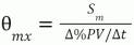
The dead time from a measurement sensor resolution or threshold sensitivity limit (Θmx) can be approximated as a measurement sensitivity limit %(Sm) divided by the rate of change of the process variable (Δ%PV/Δt). For fast and large disturbances, this dead time is negligible.
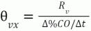
Similarly, the dead time from the control valve or VFD resolution limit (Θvx) can be approximated as a valve or VFD % resolution limit (Rv) divided by the rate of change of the PID output (Δ%CO/Δt). The equation also applies to dead band from backlash or dead band in VFD settings for reversals of the signal direction. For large or fast changes, this dead time is negligible.
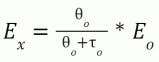
The integrated error (Ei) is the result of integrating the deviation between the process variable and the setpoint after a disturbance assuming the process variable was originally resting at the setpoint. This can be viewed as the net total area of the error on a trend recording, considering that the area of plus and minus excursions cancels out to some degree, perhaps in downstream piping and inventory tanks. In processes with back-mixing, the cancellation may occur from attenuation resulting in integrated error corresponding to the net amount of off-spec material downstream. If the oscillations do not cross the setpoint, the integrated error is the same as the integrated absolute error (IAE), which is the more common metric seen in the literature. IAE considers any deviation from setpoint as undesirable. For example, too high a flow rate means excessive filling of a package and giving away product, and too low a flow means underfilling. Alternately, too high a temperature means excessive energy use and too low means inadequate reaction rate. The advantage of the integrated error is the ability to estimate the practical limit from PID tuning settings, PID execution rate (Δtx) and signal filter time (Τf) and the ultimate limit (best theoretically possible metric) from the loop dynamics. The following equation to estimate the integrated error practical limit is obtained from the original equation by Shinskey by converting the change in percent PID output required to reject a disturbance to the percent open loop error (Eo), which is the error from a disturbance if the loop is open (PID is in manual).
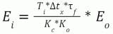
The integrated error cannot be less than what is possible based on the total loop dead time and rate of change of the excursion determined by the open loop time constant. The equation is for a step disturbance. The effect of disturbance lag can be approximated by a filter applied to the open-loop error with a filter time equal to the disturbance lag time.
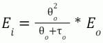
The following equation for the ultimate limit to the integrated error is based on the fact that any correction for a disturbance does not occur until one total-loop dead time has passed. The maximum rejection of a self-regulating process step disturbance is two right angle triangles, each with an altitude as the peak error and a base as the dead time to form an equilateral triangle. The approximation of the integrated error as the area of this triangle works best for a lag-dominant process. The result is the ratio of the total-loop dead time squared to the open-loop, 63% response time. For integrating processes, the open loop time constant is approximated as the inverse of the integrating process gain.
Integral of the squared error (ISE) considers that any deviation (positive or negative) is bad, and the measure of undesirability increases with the square of the magnitude. Consider that a deviation of 5 °C in a refrigerator is relatively inconsequential, but a deviation of deviation of 10 °C could cause either freezing or spoilage. During regulatory control, when the process is noisily at steady state, the ISE normalized by the time duration of integrating is equivalent to the process variance. Process variance is used to determine how close the setpoint can be to a specification or constraint, which determines the frequency of violations, quality giveaway and/or excess cost to manufacture.
The peak error is the maximum excursion in the direction caused by a load disturbance. A large peak error can cause unsafe operation, damage equipment and trigger undesirable process responses. Process onstream time is adversely affected by a peak error that causes activation of the safety instrumented system (SIS), the opening of relief valves or the blowing of rupture disks. Peak errors in waste treatment pH can cause reportable violations of Resource Conservation and Recovery Act (RCRA) limits.
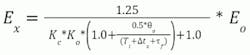
The peak error for a PID can be approximated by the following equation for self-regulating processes, realizing the second term in the denominator is usually negligible, making the peak error mostly a function of PID gain. If there is no derivative action, the numerator should be increased from 1.25 to 1.5. The equation is for a step disturbance. The effect of disturbance lag can be approximated by a filter applied to the open-loop error with a filter time equal to the disturbance lag time. For near and true integrating processes, the peak error can be estimated by multiplying the ramping open-loop error (ΔEo/Δt) by the arrest time (time to stop the initial excursion from a disturbance proceeding in the same direction) that can normally range from one dead time for aggressive control to 5 dead times for robust control. The arrest time is much larger when it is maximized, for maximum absorption of variability (for example, surge tank level control).
The ultimate limit to the peak error is the altitude of a right triangle that is the ratio of the total-loop dead time to the open-loop, 63% response time as discussed for the ultimate limit to the integrated error. The approximation works best for a lag dominant process. For dead-time dominant processes, the peak error approaches the open loop error. For near integrating processes, the open loop time constant can be approximated as the inverse of the integrating process gain.
The minimization of changes in PID output in response to noise, resolution limits, and deadband is important to prevent wear of valve packing and upsets to other loops. It is best to reduce the source of these problems by better design and installation.
If the source of noise cannot be reduced, the filter must minimize the introduction of a secondary time constant to achieve the desired reduction in output changes. Often not considered is that changes in the PID output well within the resolution limit and deadband do not actually translate to valve movement and wear. Not realized is that for integrating processes with a high PID gain permitted for tight control, the noise may seem insignificant when looking at the process variable but greatly upsetting when looking at the PID output. Also, integrating processes are very sensitive to secondary time constants that would often be the conventional first-order filter time. The second order and moving average filters can greatly reduce the dead time introduced to achieve a desired reduction in the total of unnecessary PID output changes.
The minimization of changes in PID output in response to disturbances is important to prevent resonance with loops whose oscillation period is close to the ultimate period of the subject loop and to maximize absorption of variability, which is a common requirement for surge tanks and other loops. The minimization of manipulated variable changes in response to disturbances slows down the upsets to other loops and a more gradual approach to an optimum to help prevent violation of constraints and the risk of undesirable consequences. Variable tuning based on deviation from setpoint with “mild” tuning for variability absorption when close to the setpoint and more aggressive tuning when far from the setpoint can help achieve both objectives. However, the product of the reduced PID gain and reset time must be greater than four times the inverse of the integrating process gain to prevent slow-rolling oscillations.
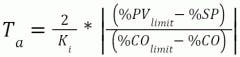
The arrest time (Ta) to maximize the absorption of variability (minimization of transfer of variability) for integrating processes particularly critical for surge-tank level control can be estimated as follows based on PV limit (%PVlimit) (for example, maximum or minimum PV that prevents activation of alarm or SIS) closest to setpoint and CO limit (%COlimit) (for example, PID output limit) closest to current output [5]:
The online metrics from key performance indicators (KPIs) developed in the digital twin and deployed in the actual plant must be converted to dollars of revenue and dollars of cost and totalized over a month. Online metrics on process efficiency, often expressed as raw material mass or energy used per unit mass of product, must be multiplied by the production rate at the time and the cost per unit mass or energy used to get dollars of cost per unit time. Online metrics on process capacity must have a production rate multiplied by the price of the product(s) sold. This is best accomplished by getting an accounting representative to participate in the development and use of the metrics.
An improvement in a unit operation performance may have a negative impact on another unit's operation. For example, a decrease in steam generation from a waste furnace from more efficient operation decreases the steam available for power generation. Rapid changes in raw materials or energy usage may upset the headers and systems that supply other systems. The online metrics must be extended to all unit operations affected to quantify the trade-offs.
The raw material and energy used do not have an immediate effect on the product produced. There are transportation and mixing delays and time constants associated with volumes and mass transfer and heat transfer rates. Transportation delays for plug-flow volumes and time constants for back-mixed volumes are inversely proportional to flow. There are tuning, dynamics and valve and measurement rangeability limitations that are often not recognized and included.
Operators are fundamentally reluctant to relinquish manipulation of process inputs and operating points if the benefits are not seen or understood. Operators may also be initially opposed to indications and comparisons of their performance. Using results in a positive way allows operators to take more ownership of process performance.
A running average, also known as a moving average over a representative period, can reduce noise and inverse response and provide a more consistent response to changes in process performance. In a running average, the newest value of the metric replaces the oldest value. For large periods, a dead-time block with the dead-time set equal to the period of the running average efficiently saves old values.
For synchronization of process inputs and process outputs, the process inputs should be passed through a dead-time block and filter block to handle process or automation system delays and lags, respectively. The dead-time and lag-filter-block settings will vary with the relationship between each input and output and is often a function of production rate or batch time. Metrics should be filtered with a time constant that is less than 1/5 of the synchronization time (dead time and lag) to reduce inverse response and noise for the shorter periods. Periods should be at least twice the synchronization time. To provide an analysis of batch operations, the period should be the batch cycle. For continuous operations analysis of operators, the period should be a shift. The comparison of shift performance can be both enlightening and motivating, stirring the natural inclination of competition. Since operator shift change is often the time for greatest disturbances and changes to operating points from personal preferences as to modes and setpoints, the recognition of shift performance can be particularly beneficial. Using a running average will show the effect of a change in performance at the beginning of a shift and for the whole shift by the sliding window of time. For real-time accounting, an accounting period is used (for example, month). For alerting operators as fast as possible to the consequence of actions taken (for example, changing PID setpoint or mode), the period can be reduced to be as short as six times the total loop dead time. The metrics at the end of a month, batch, or shift are historized.
Russ, what are the major options in process optimization?
Russ: Once we have the process models, we can use them to optimize process design, control system design, PID tuning, supervisory determination of process setpoints, and more. The optimization could be human-guided choices, creativity and intuition led by results from prior exploration. Alternately, the search for the best could be automated or algorithmic. Where alternate concepts or where numerical values are being considered, human-guided and automated optimization, respectively, is preferred.
In process design we seek to minimize costs and expenses, to maximize productivity and flexibility, to minimize resource use and pollution, etc. Rely on humans to make choices for equipment type, structure, and choices, then once a design is postulated, use algorithms for numerical values (such as size, temperature, pressure).
In control system design, let the humans postulate a control structure (for instance just feedback, or with ratio, or with feedforward). Then use simulation of the controlled process with diverse upsets and setpoint changes (using a digital twin), to observe the several metrics of performance, and let an algorithm seek the best numerical values (e.g., best PID parameters and setpoints) to optimize control system performance. One objective would be to minimize PV and controlled variable (CV) variance to be able to operate with setpoints closer to specifications and limits, which can be translated to increased throughput, lower utility costs, reduce waste, etc.
To optimize process setpoints, use the steady state model for continuous processes and an automated algorithm to search for the numerical values that provide the economically best operation. For batch processes, the translation of controlled variables to be batch slopes offer a pseudo steady state.
There are many optimization algorithms. Linear programming is fast when the objective function and constraints are linear. This is very useful for scheduling and allocation. For nonlinear constraint-free responses, the Levenberg-Marquardt algorithm is historically well-accepted; and with constraints, Generalized-Reduced-Gradient is very popular. However, in modeling and design of plants and control systems—and in plant-wide optimization—the response and constraints are nonlinear and may often have discontinuities, the numerical method for solving the model will generate striations on the surface that misdirects many optimizers, and many optimizers will get stuck in local traps. My preference is leapfrogging, a multi-player algorithm that can handle such issues. Visit www.r3eda.com for an explanation and demonstration software.
Greg: See the Control Talk column “How to optimize processes to achieve the greatest capacity, efficiency and flexibility” for some insights on optimization including the value of Leapfrogging.

3-1 Make sure the maximum deviation by disturbances from you goal is acceptable by making more immediate and aggressive corrective action (maximize proportional action to minimize peak error)
3-2 Make sure the maximum accumulation of bad conditions from a disturbance is minimized by immediate and persistent corrective action (maximize proportional and integral action to minimize integrated error)
3-3 If there is a wide range of permissible deviations from your goal, minimize disruption by corrective actions that still keep deviations acceptable (minimize transfer of variability from PV to PID output often used in surge tank level control)
3-4 If people or system response tends to ramp, be more proactive including some overcorrection to turn things around (some overshoot of FRV is needed for integrating processes)
3-5 If people or system response tends to accelerate, be more proactive including more overcorrection to turn things around (aggressive overshoot of FRV is needed for runaway processes)
3-6 Minimize the lag and delay in recognition of deviation from your goals (minimize sensor lags and delays, and make transmitter and PID filters and execution and update rates faster)
3-7 Minimize the delay in systems and people to reduce deviations from your goals (reduce process dead time)
3-8 For abnormal situations when response needs more intelligence than correction based on seeing results, suspend correction based on deviation and schedule more predictive corrections that are proven to provide recovery (use procedure automation)
3-9 Measure the “before” and “after” conditions made by corrective actions (use “before” and “after” process metrics for process control improvements)
3-10 Quantify the value of better conditions to help prioritize and justify efforts (quantify dollar benefits of process control improvements)
About the Author

Greg McMillan
Columnist
Greg McMillan retired as a senior fellow at Solutia Inc., now a subsidiary of Eastman Chemical, in 2002. He was an adjunct professor in Washington University Saint Louis’ Chemical Engineering Department 2002-04, and retired as a principal senior software developer at Emerson Automation Solutions in 2024.
