When to use controller output signal characterization
If the process gain makes large changes over the operating range, then tuning PID (or other linear) controllers is difficult. If tuned for one region, the controller is undesirably sluggish or aggressive in another.
The change in the process gain may be the result of any of several process or equipment features. One reason could be operation rate, or throughput. At high rates, typically, larger control action is needed to effect control of temperature, composition, etc. At high rates, then, the process sensitivity to control action, the process gain, is lower. In this example, the gain is due to, or characterized by, operating rate.
A second classification reason for gain change might be the operating setpoint. For instance, if a distillation purity setpoint is increased, then changes in purity are less sensitive to control action, which means that process gain diminishes. Or, consider pH control; classically gain is very high when the pH setpoint is near neutrality, but very low in the acidic or caustic region. In these examples the gain change is characterized by the setpoint.
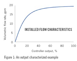
Finally, third, in some cases the process gain is due to, or characterized by the controller output. For example, if the inherent characteristic of a flow control valve is not matched to the flow process conditions, the process gain, the steady state flow rate associated with controller output, is not linear. Using Equation (3) from my August 2020 article in Control (“Understanding valve characteristics,” p41), Figure 1 illustrates how steady state flow rate could respond to controller output (valve position) when a linear valve is installed in a line. In this particular example, over the intermediate operating range of 5 to 18 gpm, the process gain changes by a ratio of 95:1, which makes controller tuning difficult.
In these three cases, gain scheduling of the controller is a reasonable solution—tune the controller for the several operating conditions (high, medium, and low operating rate or setpoint), place the desired tuning values associated with the flow rate or setpoint in a look-up table, and transfer those values to the controller when the conditions change.
However, where the static nonlinearity can be characterized by the controller output, and the process dynamic response remains relatively unaffected, output characterization is the recommended solution to linearize the loop response, to create a constant loop gain, and solve the tuning problem.
In this technique, the output signal from a controller, ϲ, does not go directly to the final control element. Instead, ϲ is transformed to an alternate signal υ, which goes to the final element. The term transform means algebraic signal conversion, a simple function, not a Laplace transform. This is illustrated in Figure 2. As ϲ goes from 0 to 100%, υ also goes from 0 to 100%, but it is not a linear relation. In this illustration when ϲ is at 50% υ is only at about 20%.
The output characterization signal conversion will have the inverse shape of the process response to the controller output. In Figure 1, the shape is square-root-ish. If you were to switch the two axes and plot controller output with respect to flow rate, the graph would appear quadratic-like, which is the shape illustrated in Figure 2. However, the signal conversion has the units of percent to percent, not the process variable units.
This article is about how to get the inverse relation for the output signal transformation. I’ll present two methods. One is using an algebraic functional conversion, and the other is using a piecewise linear transformation. Both are grounded in the same compensation concept.
Concept for output characterization
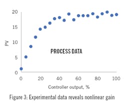
Either do experiments or use the historian to obtain steady state data for values of the process variable of interest with respect to the signal to the process. Set the output of the controller, the signal to the process, which means that ϲ = υ, wait for steady state, and record the process variable (PV). This would represent Figure 1, but rather than a continuum line from a phenomenological model, you’ll have discrete data points, which are affected by noise and other sorts of experimental process variability as well as calibration offset in all of the control system devices (D/A. i/p, valve actuator, measurement, A/D). If possible, include the full range of controller output, ϲ. If not, extrapolate to 0 and 100%. The data may look like that in Figure 3, but you might not have so many data points. Notice the experimental variation. Also notice the zero offset. In some processes, if ϲ is zero the PV should be zero, but calibration errors will make it other. And, in many processes the minimum PV value is not zero (consider temperature or pressure).
Second, scale the PV value to a percent of full range, ρ, using the following relationship:
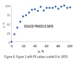
Perhaps plot ρ against the signal to the process, the ϲ = υ, as in Figure 4. The graph is not necessary, but it may be instructive.
Figure 4 should have the same appearance as Figure 3, except that the vertical axis goes from 0 to 100% and there is no zero offset--when υ = 0, ρ = 0.
What we would like is a linear PV response to controller output: When the controller output is 50% the process is also at 50% of full range, and 23% matching 23%, etc. But in Figure 4, when the process is at 50%, the controller output is a bit less than 20%. We would like a formula that changes the 50% controller signal, ϲ, to a bit less than 20%, υ, so that when the υ = 20% goes to the process, the PV response is 50%. This would be the output characterization formula in the block in the middle of Figure 2.
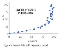
To get such a formula, third, switch the axes of Figure 4, and recognize that the ρ is the desired controller output, ϲ. See Figure 5. Notice that the shape in the relation of Figure 5 is the inverse of the process response. Notice that υ is the signal to the process from the data generation experiment, and that the horizontal axis is ρ, now the desired value of ϲ. In the experiments, υ = ϲ, but what we want is ϲ = ρ.
Now, fourth, use any favorite technique to generate an equation to calculate υ from ϲ. The dashed curve in Figure 5 shows one model.
Mathematical inverse function method
If you are lucky, classic trendline fitting will generate a good relation for the data in Figure 5. But in this case, quadratic, cubic or other power law or polynomial models do not give a good fit. Neither do exponential, logarithmic or many other simple modeling techniques. So, I chose to derive a model structure that seems to fit the data. I looked at the trend in Figure 4, supposed that it could be represented by an exponential model (which is not the truth about the relation), then inverted the model to obtain:
and found the α and β values to best fit the data. The dashed line is the model that is used to convert ϲ to υ, the output signal conversion block function in Figure 2.
If you have a first principles model of how the PV should respond to ϲ, and can algebraically invert it, then such might be an excellent model for this output transformation. But since there is no requirement that the process must comply with an ideal first-principles model, you will likely have to adjust model coefficients to make it best fit the data.
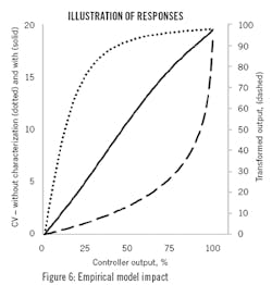
In any case, the empirical model is not a perfect fit to the data. Note in Figure 4 that it is a bit above the data in the mid output range and a bit to the right of the data in the high output range. The model is not the perfect inverse, it is an approximation.
Figure 6 shows the results when the output characterization model is used to convert the controller output, ϲ, to the signal to the process, υ. The dotted curve represents how the process (left-hand vertical axis) responds to the controller output without the signal conversion, basically representing Figure 1. The dashed curve is the inverse model (of Figure 5), which is used to convert the controller output to the signal to the process (use the right-hand vertical axis). The solid curve in the middle is the process response (left-hand vertical axis) to the controller output, with the signal conversion structure illustrated in Figure 2. Without output characterization, the gain changes by a 95:1 ratio (dotted line). With output characterization, the gain changes by a factor of about 2:1.
If the model were to be the exact inverse, the process response would be exactly linear. But an analytical model, fit to noisy process data, cannot be exactly the process phenomenological inverse.
Now that the gain is nearly constant, tuning the controller will be easier.
Piecewise linear inverse method:
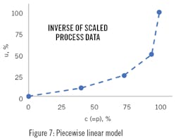
It may be nearly impractical to obtain a single algebraic function to convert ϲ to υ. In many cases modeling the trend in Figure 5 with a piecewise linear (connect-the-dots) relation is simpler and fully adequate. Figure 7 illustrates a piecewise linear model. First, select points that, when connected with straight lines, the connect-the-dot lines still adequately match all of the data. I chose 5 points; another person might have chosen 4 or 6 points. The choice is not critical as long as the connect-the-dots model generally matches the inverse data of Figure 5. The points are not equally spaced, but should include 0 and 100%. The break-points for the piecewise linear model do not exactly match any of the data. Instead, I selected break-points to represent a local middle of the data. (Similarly, the regression model does not exactly go through each experimental data value.)
The piecewise linear model is relatively simple. Your system may have an f(x) block that does this for you. If not: Label the points with an index ι = 1,2,3,4 ... from lowest to highest. Between points use a linear model to convert ϲ to υ:
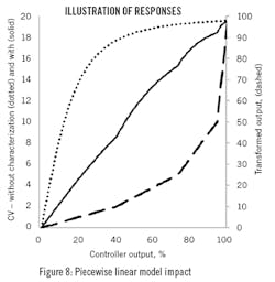
Figure 8 shows the results using the piecewise linear model as the output characterization. Similar to Figure 6, it shows the non-converted response (dotted) and the transformed response (solid). Note in this case the conversion model (dashed line) is piecewise linear. It has slope discontinuities at the break points.
With the piecewise linear output characterization, the gain changes by a factor of about 3.5:1. Again, if the model were to be the exact inverse the process response would be exactly linear. But, any sort of empirical model fit to data is not exactly the process phenomenological inverse.
Again, now that the gain is nearly constant, tuning the controller will be easier.
Perspectives
This case, illustrated with a process with a 95:1 gain ratio, is quite extreme. But either modeling approach reduced the gain ratio by a factor of about 35. Neither modeling approach is more right than the other. If there is a simple functional relation for the inverse model, use it. If not, use a piecewise linear model.
Balance sufficiency with perfection. A greater number of experimental data pairs, or a more complicated model will more perfectly linearize the MV to PV response. But, it takes more time to get a more perfect model, and then, greater effort for your successor to manage it. Many times, a simple regression model or two intermediate points are all that is needed.
Output linearization compensates for gain changes, the steady state relation between controller output and PV. If the process dynamics (deadtime or time-constant) also change with the signal to the process, you still might need to gain schedule the controller with tuning coefficient values appropriate for each range.
Gain scheduling requires separating the operating range into local regions of similar process gain, then tuning the controller for each. That may be three or so tuning tasks. If you can adequately linearize the loop with output characterization, then one tuning activity is all that is needed.
Input signals can also be characterized. The most common application of an input signal characterizer is for pH control. Here we start with a titration curve obtained from lab titration of a process sample at operating temperature and concentration. The titration curve must have at least 10 data points on the steep part of the curve and in the operating region. A theoretical curve obtained from even the best electrolyte modeling program needs to have the concentration of weak acids and weak bases and conjugate salts adjusted so that the slope (process gain) in the control region of the computed curve matches that of the actual titration curve from the lab titration. Small amounts of carbonic acid absorbed from seemingly insignificant amounts of carbon dioxide in the atmosphere can decrease the slope of a strong acid and strong base system by several orders of magnitude. The use of lab titration curves at actual process conditions is critical. Make sure operators, engineers and technicians can see and help maintain the characterizer performance. For this reason, signal characterization is best done in the controller configuration than in the field.
Besides the obvious benefit from a more linear process gain, the characterizer can restore the identified process time constant. In a worst case scenario, a 19 minute time constant would be reduced to a 0.04 minutes for a pH approaching neutrality (7 pH) in a true strong acid and strong base system. The acceleration in pH response can resemble a runaway response to the PID controller until the process slows down on the extremely flat extremes of the titration curve causing a cycle (e.g., 2 to 12 pH). The characterizer eliminates the acceleration and need to detune the controller for the steepest part of the titration curve. The resulting higher controller gain enables a higher rate of change of controller output that gets through control valve resolution limit quicker reducing deadtime. The amplitude of a limit cycle from a resolution limit (stiction) is also reduced since it is proportional to the process gain. The benefit is similar to that obtained for a valve by linearizing a quick-opening type of installed flow characteristic.
The implementation of input and output signal characterizers generally increases the time constant to deadtime ratio and decreases a limit cycle amplitude improving loop performance. The identification of the open loop gain, time constant, and deadtime is less dependent upon the setpoint and the size and direction of the change in controller output. The identification of dynamics becomes more consistent.
Processes change in time. Piping paths are re-routed, new or alternate devices installed, in-line screens are partially blocked, heat exchangers foul, catalysts deactivate. All such changes affect the process gain. The model that you devise with data on one day, may need to be changed when the process changes. Keep it simple.
Author's acknowledgement:
I appreciate the review and commentary from Jacques Smuts, OptiControls, Inc. and Gregory K. McMillan, Control Talk columnist as I prepared this article.
About the Author
R. Russell Rhinehart
Columnist
Russ Rhinehart started his career in the process industry. After 13 years and rising to engineering supervision, he transitioned to a 31-year academic career. Now “retired," he returns to coaching professionals through books, articles, short courses, and postings to his website at www.r3eda.com.

