Using feedforward control to deal with disturbances

If a disturbance is measurable, then its measured value can be used in feedforward control to prevent the disturbance from upsetting the process.
Feedback (PID, etc.) is like reactive maintenance. After you see the problem, start fixing it. By contrast, feedforward is like predictive maintenance. When you anticipate there will be a problem in the future, take action to prevent the problem from happening so it does not happen.
The “D” action in PID is anticipatory, but not in the feedforward or predictive sense. It leads the actuating error to anticipate what the error might become soon. This is not feedforward. PID looks at the actuating error, the deviation from set point, which is the process response to a disturbance. The evidence of a disturbance is not seen until after it starts to be expressed by the process. Even with “D” action, feedback does not respond until after the disturbance begins to show its effect on the process. Feedback looks at the process response, the present consequence of the past disturbance.
By contrast, feedforward looks at the disturbance variable, the cause of the future process deviation, not the actuating error. Feedforward acts before the actuating error would indicate action is needed.
An example by analogy
As a human example: It was chilly in the morning, so he wore a jacket. A while after the sun came up, he started sweating and took off the jacket. That was feedback. The corrective action (removing the jacket) came after the problem (sweating, too high of a body temperature) was sensed.
On the other hand, seeing the sun rising and knowing what would eventually happen, take off the jacket just prior to being uncomfortable. It is feedforward action is taken before the actuating error indicates it is needed.
Feedforward model coefficients
There are four coefficients in feedforward control (the action is often termed a dynamic compensator). The most important are delay and gain, which are also the easiest to determine.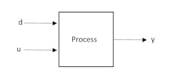
The process model for feedforward control
We consider the process with output, y, being affected by both the measurable disturbance, d, and the controller MV, u. As illustrated in Figure 1, the process may be a reactor with yield as the output, y, with raw material composition the disturbance, d, and the controller signal to the reagent valve, u. Alternately, the process may be distillation with distillate composition, y, being affected by both column feed rate, d, and the signal, u, to the reflux flow control valve.
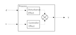
Both d and u affect y. Conceptually, as illustrated in Figure 2, from step tests in d and u one can get FOPDT models for how y responds to either d or u.
However, one does not need single perfect steps from an initial steady state to a final steady state. I believe that experience could provide reasonable estimates for the gain and delays, and perhaps even the lead and lag.
Without such experience, I recommend using regression on multiple input changes, which do not need to be steps. The input changes might also be what naturally happens. However, when getting the response to the disturbance, keep the controller in MAN with a fixed output, or else the control action will confound the response. When getting the process response to the controller MV, make sure that the MV changes are large enough to overshadow the naturally occurring d impact on the CV. My FOPDT regression program [1] can be used to convert I/O data to the models.
Determining feedforward action
Intuitively, it is easy to determine the feedforward delay and gain from process response models. As illustrated in Figure 2, the delay for the process to show the impact of the disturbance is 7 min, and the delay for the process to express the impact of the MV is 4 min. Then the MV should respond to the d at 7-4=3 min after the d changes. This rule is θff=θd-θu.
If the gain of the disturbance impact on the process is 5 [CV/%] and d makes a +2 [%] change then you expect the eventual process response to be +2*5=10 [CV units]. So, the MV needs to have a -10 [CV units] impact to cancel the d impact. If the gain of the MV impact on the process is 6 [CV/%] then, to create the needed -10 [CV units] impact, the MV needs to move -10/6=-1.67 [%]. This rule is Kff=-Kd/Ku.
Both rules are from intuitive logic. As we’ll see they are also outcomes of mathematical analysis, the lag and lead can be intuitively chosen also, but the logic is a bit complex. However, mathematical analysis of a model of the system can lead to gain, delay, lead, and lag values.
To mathematically derive the feedforward action, use a simple concept that the u and d effects on the process are independent and additive. This model is illustrated in Figure 3.
Using FOPDT models for how y is affected by u and d, in Laplace notation, the concept of Figure 3 is this mathematical model:
y=(3e-7s/10s+1)(d)+(3e-4s/7s+1)(u)
We want to determine u such that the change of y is zero when d changes. So, set y=0:
0=(Kde-θds/τds+1)(d)+(Kue-θus/τus+1)(u)And solve for u. Although the abstraction of Laplace is difficult, the algebra is easy. The answer to how u should change is:
u=-(Kde-θds/τds+1)(τus+1/Kue-θusd=-(Kd/Ku)e-(θd-θu)s(τus+1/τds+1)d
u=Kffe-θffs(τlead, ffs+1/τlag,ffs+1)d
With data from the two FOPDT models from Figure 2:
θff=θd-θu=7min-4min=3 min
Kff=-Kd/Ku=-(3y_units/d_unut)/(3y_units)(u_unit)=-1(u_units/d_unit)
τlead, ff=τu=7 min
τlag, ff=τd=10 min
In this case, the rule is, “Add the following action to whatever the feedback controller wants to do: When d makes a change, wait θff=3 min before changing u. Make the change in u be Kff∆d=-1(u_units)/(d_unit)∆d. But don’t implement the entire change now, jump to τlead, ff/τlag, ff=7 min10 min=0.7 of the ultimate value. Then lag to the final value with τlag, ff=10 min.”
Characteristic of Laplace analysis, this analysis is in deviation variables. The change in the disturbance from a base value determines the change in MV.
∆u=Kff∙∆d
The action is not based on the disturbance value, but its deviation from a base or reference value.
Include feedback control
- We still need feedback control. There are several reasons:
- Feedforward can only fix the measurable disturbance. Other disturbances will still affect the process. Feedback is needed to fix the others;
- The feedforward model is not perfect, it is an FOPDT approximation. So, although feedforward help will be very good, it will not be perfect. Feedback is needed to trim the feedforward imperfection;
- If the disturbance measurement is in error (perhaps due to calibration drift), then the feedforward correction will be imperfect. Feedback is needed to compensate; and
- Feedforward cannot move the process to a new set point. Feedback is needed to do that.
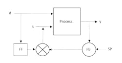
Typically, feedforward control action is added to the feedback action with a control structure illustrated in Figure 4.
Here is the issue: If the FB action is 90% and the FF action is 20% then the combined 110% is infeasible. Only 100% can go to the process. (Figure 4 does not show the override from the summation circle.) The override causes an effect similar to wind up. If the FB controller wants to correct a CV error by lowering the signal by 5%, lowering its output to 85%, the sum is 105% and the valve remains 100% open. Nothing happens until the feedback output winds down to 79%.
If the feedforward controller is adding 20%, then the output of the feedback controller should be limited to 80%. If either using limits on the integral or external reset feedback (erf), the FF action needs to be included in the feedback bias limitation. For instance, the erf signal to the feedback controller must be adjusted for the FF contribution.
erf=MVactual-FF
The control device should take care of all this for you. You need to determine the four FF coefficient values: θff, Kff, τlead, ff, and τlag, ff.
Illustration
First, here is an illustration of feedback alone.
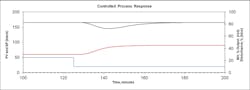
Figure 5 illustrates a tuned PID feedback controller (MV is the middle trace) with no feedforward action reacting to a disturbance (the lower step change). The CV and SP are the upper traces.
Notice: The control action does not start until after the CV deviation is visible. When the deviation is small the control action is small, even though it eventually needs to be much larger. The “D” action in the PID controller does not anticipate what the fully developed deviation will be.
Second, Figure 6 illustrates the same feedback controller and same disturbance, but with feedforward.
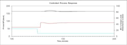
Even a simple FF without lead and lag can be a very good prevention. Figure 7 illustrates the same situation but with both τlead, ff and τlag, ff set to zero.
Quality giveaway
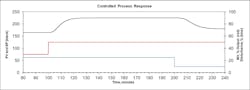
How can you quantify the benefit of feedforward? Here is one method. Figure 8 illustrates the process in regulatory mode. The dotted line at the CV value of 200 represents the CV limit—perhaps a customer specification or a safety or operational limit. The process set point at 185 is 15 CV units lower than the limit. The disturbance continually causes deviations from the SP, which are countered by the well-tuned feedback controller. There are only occasional and very small PV violations of the limit. But if the set point is increased, closer to the limit, there will be many and significant violations of the limit.
We would like to have the set point closer to the limit. The 15 CV units deviation between set point and limit is termed quality giveaway. Consider that the CV represents impurity and 200 is the specification (maybe the units are ppm). Then if the set point was at the specification there would be many unacceptable purity deviations. In this example, to prevent purity violations, one must manufacture on average a product that is 15 units purer than required. Higher purity requires greater energy input, or more culled product, or slower production, or some other operational aspect that can be converted to manufacturing costs. Process owners should be able to quantify such costs.
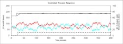
Notice: There is much reduced variation in the CV. At no time is the CV close to the limit. The MV (red trace) is a mirror image of the disturbance (blue trace) but with a bit of a delay.
Now that control is greatly improved, the set point can be closer to the limit. In Figure 10, the set point is just five quality giveaway units from the specification. There are no violations.
Takeaway
If a disturbance source is measurable and has a dominating impact on the CV, then feedforward action can be a substantial benefit to regulatory control.
Implement feedforward within the manufacture’s devices so that integral wind up, initialization, and MAN-AUTO transfer issues are properly handled.
You don’t need perfect models. Often just intuitive values for feedforward gain and delay, and zero for the lead and lag time-constants, will provide substantial feedforward benefit.
You don’t need to determine models from ideal step tests. Regression can be very beneficial in fitting models to data.
Feedforward assists feedback. It is not the primary signal to the final control element. It trims the feedback controller signal based on disturbance deviations from a base value.
You still need feedback control for set point changes, compensation for measurement errors, feedforward model errors, and other disturbances.
Russ Rhinehart started his career in the process industry. After 13 years and rising to engineering supervision, he transferred to a 31-year academic career. Now “retired”, he enjoys coaching professionals through books, articles, short courses, and postings on his web site www.r3eda.com.
About the Author

R. Russell Rhinehart
Columnist
Russ Rhinehart started his career in the process industry. After 13 years and rising to engineering supervision, he transitioned to a 31-year academic career. Now “retired," he returns to coaching professionals through books, articles, short courses, and postings to his website at www.r3eda.com.
