Variations in the PID algorithm
When tuning a control loop or choosing an algorithm version that's consistent within your use context, it's important to understand the variations that exist in the proportional, integral, derivative (PID) algorithm. Unfortunately, there are many names for the several key versions of the algorithm, and names such as series or parallel are each applied to two distinctly different formulations. Accordingly, it's been best to identify the algorithm formulation by its calculus or Laplace representation, not the many names, to make clear distinctions.
To help unify the nomenclature, ISA Standards Committee 5.9 is suggesting uniform naming conventions for PID algorithms. This article is intended to update the reader on the committee’s current agenda, as well as reveal some of the commonly applied alternate names that you may be using.
The main three PID algorithms
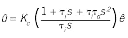
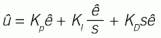
Standard: a Laplace representation of the standard algorithm is: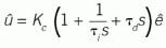
This has been called parallel because the block diagram has the P, I and D operations in parallel. But it's also called series because in this mathematical form the controller gain multiplies each of the P, I, and D terms in series. It's called ideal because 1) it's the form that arises from controller synthesis and 2) it's the most convenient for mathematical analysis. It's been called the ISA standard, even though ISA hasn't declared any algorithm as such. It's also called non-interacting, or non-interactive, perhaps because it lacks that feature of the interacting controller. The ISA 5.9 committee is moving toward recommending this form be called “standard,” but not declaring this as the best or right way to formulate the P, I and D functions.
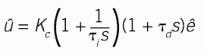
There are many versions of how this standard equation can be represented. If the terms inside the parentheses are combined, then it will appear as: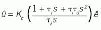


Although it appears different in these alternate mathematical representations, there is no new functionality. I showed proportional band and reset rate together, although they can be independently applied.
Parallel: If the controller gain and actuating error are multiplied onto each term in the parenthesis, and coefficients combined, the standard form becomes:
Again, there is no alternate functionality, just P, I and D. This version has been given multiple names. Independent gains because of the three gains, and parallel gains or just parallel because of the structure. The ISA 5.9 committee is moving toward recommending this form’s label as “parallel.”
The translation of tuning coefficients between “standard” and “parallel” forms is straightforward. For example,

So, if you have tuning rules for one, the translation to the other is simple. However, I think that it's best practice for an operating unit to choose one algorithm version to prevent confusion, and standardize operational and tuning procedures.
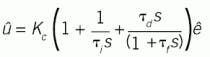
Series: I was raised calling this the rate-before-reset version:
This too can be mathematically factored in many ways. Here the

term is the leaded actuating error, a projection of what the actuating error is anticipated to become,

Then the P and I operations are on the anticipated error,
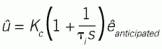
In a block diagram, this calculates the rate before the integral (often termed the reset function), hence the rate-before-reset name. But the block diagram also suggests the name series because the rate term (as a lead) happens prior to the integral. It's alternately known as the physically realizable controller because this is how D was added to PI functionality in the mechanical-pneumatic device era. If you multiply the two binomials and collect common terms, then the Laplace formulation becomes:
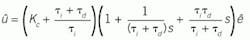
This representation reveals the interaction of terms. If you adjust the derivative action, it also adjusts the P and I term coefficients. So, it's often termed the interacting or interactive version. Interacting as a controller description seems to convey a desirable feature, but I think the interaction is really a confounding attribute. Note again, there is only the P, I and D functionalities. ISA 5.9 is moving toward recommending the label “series” for this form. Again, if you have tuning rules for either the “standard” or the “parallel” forms, you can translate values to the “series” form. However, it's not so simple to convert the series coefficient values to the standard (you need the quadratic formula).
Note that, in spite there being several PID versions, all have, and only have, the same three functionalities of P, I and D. One controller version is not functionally better than another, but there are many ways to present the controller terms. So, for tuning, the user needs to know exactly how the vendor has structured the algorithm. Also, the ISA 5.9 committee is moving toward recommending this nomenclature, but ISA has not yet declared any terminology as standard.
Other PID modifications
There are many other embodiments for each of these three PID versions. These include:
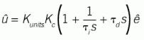
Velocity mode, which calculates incremental changes to the MV, not the MV value. In calculus notation for the standard controller: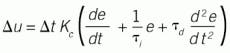
When tuning, you need to be aware what options are selected to be sure that the modification is compatible with the method. For example, if part of tuning is to make step changes in the SP, you must remove setpoint softening features and choose P-on-e.
Other control algorithms
There are many alternate control algorithms to the basic PID controller. PID evolved in the mechanical-pneumatic, pre-electronic days. Mechanical devices were replaced by analog electronic devices, and then by digital devices. Digital devices permit more sorts of calculations than just P, I and D and first-order filters. Some control techniques permitted by digital computers include:
- Model-based control (MBC), alternately called horizon predictive control (HPC), dynamic matrix control (DMC) or advanced process control (APC). This method traditionally uses linear vector impulse models of the process and optimization to find the best sequence of future control actions to move the CV toward the setpoint, while avoiding constraints. It can handle multiple input, multiple output (MIMO) processes, and includes delays and feedforward action. Typically, the models are linear (fixed and uniform gains) and stationary (fixed time constants and delays). This has gained traction in the process industries, and many vendors offer their own version and range of options.
- Modern control is alternately called state-space or ABCD matrix model-based control. It's also linear, stationary and MIMO. In addition, it's gained traction in aeronautical and electronic applications.
- Generic model control (GMC). When the model is a steady-state SISO model, this reduces it to PI control with output characterization (inverse of the SS model). The benefit is when processes are nonlinear, they effectively have no or little delay, and time-constants don't change. I believe this can be easily implemented by in-plant engineers in standard devices, and that using first-principles models has other benefits for those managing processes.
- Predictive functional control (PFC) uses a model of the process to forecast what the process might do in the future in response to an MV change. The model could be a traditional linear model or a first-principles, nonlinear model, which includes disturbance and nonideal transient effects. In any case, the MV value is selected to get the modeled value to match the SP value at some future time, the coincidence point. There's only one tuning value per CV, the future time of the coincidence point, which is placed beyond the delay or inverse action. These attributes provide many user benefits—tuning simplicity, robustness to ill-behaved dynamics and/or nonlinearity.
- Process-model-based control (PMBC) was developed as a one-step-ahead, model-based controller to use the process engineer’s first-principles model of the process. It also includes a method to incrementally adjust model coefficients values to keep the model true as process behavior changes. The single tuning coefficient per CV is the desired initial rate of the process returning to the setpoint. The adapting model can be valuable in both process monitoring and constraint adjustment in supervisory algorithms.
Bottom line, it's important to understand how your controllers were set up by others and which versions and modifications are best within your application context.

About the Author

R. Russell Rhinehart
Columnist
Russ Rhinehart started his career in the process industry. After 13 years and rising to engineering supervision, he transitioned to a 31-year academic career. Now “retired," he returns to coaching professionals through books, articles, short courses, and postings to his website at www.r3eda.com.
