When a digital twin’s model coefficient values are adjusted in real-time, noise, digitization, spurious signals and other data features can lead to unwarranted changes in model coefficient values. This is termed tampering, a statistical process control (SPC) label coined by W. Edward Demings to mean adjustment in response to noise—to a phantom indication—not to a true need for adjustment. Tampering increases variability, costs energy, increases wear and adds confusion.
This is Part 3 of a three-part series on understanding the digital twin. Part 1 defined a digital twin as a model of the process that's frequently adapted to match data from the process. This keeps it useful for its intended purpose. Part 2 discussed how to continuously adapt the model with online data, while this Part 3 discusses tempering adaptation in response to noise.
In the context of process model adjustment, data features such as process noise, signal discretization, spurious values, etc., perturb true process values. This can cause an algorithm to make a model coefficient value adjustment, even if no adjustment was justified. An SPC cumulative sum approach can be used to temper such adjustments. That is, to only permit coefficient adjustment when there's statistically significant evidence that adjustment is warranted. This approach follows that originally presented in reference [1], summarized in reference [2] and demonstrated in references [3, 4]. The rule is “Hold the prior coefficient value until there's adequate evidence to report that the value has truly changed.”
Consider that the process variable, x, is “stationary”—its mean is constant (the process is at steady conditions), and “noise” is independent, random influences added to the mean at each sampling. If the noise is normally (Gaussian) distributed, there's only a 0.27% chance that data will appear in the tails of the histogram (more than 3σ̂x from the average). (Here the hat over the σ indicates that it's an estimated value from data.) Only one out of 370 points will fall in the extreme tails.
If x really changes, then the average will shift, and there's a good chance that the new process will place points outside of the old 3σ̂x limits. The SPC philosophy is: if x is more than 3σ̂x from the old average, x̄old, then one will accept that the process really has changed. Though one will be wrong 0.27% of the time, the basic SPC philosophy is:
If |x – x̄old| > 3σ̂x, then respond (1)
But, the action from Equation (1) waits until one point is in the improbable tail region. If the process shift is small compared to σx, then it may take many points before the first measurement is more than 3σ̂x from the average. However, if there's a shift in the mean, then the measurements will show a systematic bias from the old average. So, observe evidence of a systematic bias, not just a one-time event.
Define the variable CUSUM as the cumulative sum of deviations from the reported average scaled by data variability:
If the process hasn't changed and noise is independent at each sampling, then we expect CUSUM to be a random walk variable, starting from an initial value of zero. However, if the process has shifted, then CUSUM will steadily, systematically grow with each sampling. CUSUM is the cumulative number of σ̂x's that the process has deviated from x̄old. CUSUM could have a value of 3 if there is a single violation of the 3σ̂x limit. Regardless as to whether it's a single or accumulated value of 3, for this procedure,
If |CUSUM|>3√N take action (3)
The variable N is the number of samples for which the variable CUSUM is calculated, and the square root functionality arises from the statistical characteristics of a random walk variable. The trigger value, 3, representing the traditional SPC 99.73% confidence level in a decision, is not a magic number. If the trigger value was 2, approximately representing the traditional 95% confidence level of economic decisions, then action will occur sooner; but it will be more influenced by noise: 5% of data in a normal steady process will have a ±2σx violation. If the trigger value was 4, representing the 99.99% confidence level, then the reported average will be less influenced by noise, but it will wait longer to take action. Values from 2 to 4 are generally chosen to balance responsiveness and false alarms for particular SPC applications. For data filtering, I find that the trigger value of about ±2.5σx gives desirable results. Choose TRIGGER=2.5, and:
If |CUSUM| > TRIGGER √N, then take control action (4)
The action will be to report a change in the mean of the noisy process variable. How much change should one take? Short of detailed process model inference procedures, primitively credit that x̄ had sustained an average offset since the last change in x̄. Since the previous value of CUSUM at the true x̄old was about zero, with a shift to a value of x̄new the CUSUM is now N(x̄new – x̄old)/σx.
Accordingly:
If |CUSUM| > TRIGGER √N, then
x̄new = x̄old + σx • CUSUM / N
And reset N and CUSUM to zero (5)
Since my preference is to eliminate possible instances of a divide-by-zero (which may occur if the measured value is “frozen” and σ̂x becomes zero), re-define:
CUSUMNEW = CUSUMOLD + (x – x̄old) (6)
Then the trigger is on TRIGGER σ̂x.
The method requires a value for σ̂x, and the value of σ̂x should automatically adjust when the process variability changes. Based on the EWMV (exponentially weighted moving variance) technique define:
Where M is the number of samples to be averaged to determine the variance, and λ = 1/(M – 1) is the first-order filter factor.
Then estimate the data standard deviation from Equation (7):
I find that λ ≅ 0.1 (or M ≅ 11) produces an adequate balance of removing variability from the σ̂x estimate, yet remaining responsive and having a convenient numerical value.
Including in initialization of variables, in a pseudo-Fortran language, the algorithm is:
IF (first call) THEN
N := 0
XOLD := 0.0
XSPC := 0.0
V := 0.0
CUSUM := 0.0
M := 11
FF2 := 1.0/(M-1)/2.0
FF1 := REAL((M-2)/(M-1))
END IF
Obtain X
N := N + 1
V := FF1* V + FF2*(X – XOLD)2
XOLD := X
CUSUM := CUSUM + X - XSPC
IF (ABS (CUSUM).GT.TRIGGER*SQR (V*N)) THEN
XSPC := XSPC + CUSUM/N
N := 0
CUSUM := 0.0
END IF
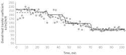
Figure 1: Trend lines show actual heat transfer coefficient (solid) vs. statistically filtered value (dotted).
Since computer code represents assignment statements, not equality, I used the “:=” EXPRESSION rather than the simple “=”.
A practical example
Consider the same heat exchanger example used in Part 2 of this series (Oct ’21, p. 35). As illustrated in Figure 1, the dashed line represents the true but unknowable value of the overall heat transfer coefficient. The open circles are calculated U-values from the process temperature and flow rate data. Variation on the data-based U-values is due to measurement noise. The solid line is the CUSUM filtered value. The initial value of about 210 is a start-up value and doesn't match the true value of about 200, but after about 25 samples, there's enough confidence to change the filtered value to nearly the true 200. Then, as the true value drops, the CUSUM filtered value periodically drops whenever there is adequate evidence. Finally, the filtered value is nearly at the true final value, and at sample 97 there's been enough evidence to justify a small upward correction.
Notice in Figure 1 that the noise amplitude in the data on the left side is about 4 times greater than that on the right side. This does not confound the CUSUM filter, because the trigger is scaled by the estimated data standard deviation. By contrast, first-order filters have a fixed time-constant, and if tuned for the high-noise region, would have an excessive lag in the low-noise region.
Notice that the filtered value holds steady until it changes. By contrast, first-order filters, or incremental adjustments, continually perturb the filtered value, which would continually perturb any calculation based on it.
Figure 2: The declining heat transfer coefficient indicated in Figure 1 may indicate performance degradation requiring maintenance.
As indicated in Part 2, tracking such a value of a process attribute can be used to forecast maintenance. Additionally, adapting model coefficients permits forecasting process constraints.
Figure 2 indicates the maximum achievable temperature limit possible, given the estimated value of the overall heat transfer coefficient. Based on the CUSUM filtered value of the overall heat transfer coefficient, the predicted constrained value doesn't continually fluctuate, but makes incremental changes only when statistically justified.
Key takeaway
Prevent process noise from continually perturbing KPI values. Rather than using the conventional first-order filter, consider SPC technique to prevent tampering.
I’ve used this technique numerous times as indicated in some of the references. Not included has been an industrial application of SPC filtering of control action based on mineral analysis (noisy with a significant delay).
References
[1] Rhinehart, R. R., "A CUSUM-Type On-Line Filter," Process Control and Quality, Vol. 2, No. 2, Feb. '92, pp. 169-176.
[2] Rhinehart, R. R., Nonlinear Regression Modeling for Engineering Applications: Modeling, Model Validation, and Enabling Design of Experiments, Wiley, New York, NY, USA (2016).
[3] Mahuli, S. K., R. R. Rhinehart, and J. B. Riggs, "pH Control Using a Statistical Technique for Continuous On-Line Model Adaptation," Computers & Chemical Engineering, Vol. 17, No 4, 1993, pp 309-31
[4] Muthiah, N., and R. Russell Rhinehart, “Evaluation of a Statistically-Based Controller Override on a Pilot-Scale Flow Loop,” ISA Transactions, Vol. 49, No. 2, pp 154-166, 2010
About the Author
R. Russell Rhinehart
Columnist
Russ Rhinehart started his career in the process industry. After 13 years and rising to engineering supervision, he transitioned to a 31-year academic career. Now “retired," he returns to coaching professionals through books, articles, short courses, and postings to his website at www.r3eda.com.


