Quantifying lost manufacturing time

Understanding asset utilization is key to maximizing productivity in any industrial process. In manufacturing, production can be held up by several sources including mechanical breakdowns, material shortages, external delays, operator errors and equipment degradation.
To evaluate operational performance, manufacturing productivity is quantified by measuring these key loss categories:
• Quality—quantified by off-specification product;
• Availability—quantified by equipment failures and material shortages; and
• Performance—quantified by slow cycles and small stops.
Data analysis plays a crucial role in automatically calculating and monitoring lost productivity because it can inform manufacturing personnel of their leading loss sources, which can be addressed as part of a continuous improvement program.
In part one of this two-part series, we’ll demonstrate how Seeq's analytics software was deployed by Syngenta—a global producer of agrochemicals—to establish phase-duration benchmarking analytics based on historized batch data, separated by phase start and end times. Using a basic set of assumptions, Seeq can be used to classify and generate insights into lost productivity without requiring operator- or equipment-provided reason codes.
Process background
This case study is derived from a chemical manufacturing process at Syngenta, in which two mixtures are combined and then held at temperature for a fixed time until they react. At the end of the reaction phase, a sample is taken to ensure the level of an unwanted byproduct is below the upper limit, so remedial treatment in a downstream unit won’t be required.
Following the reaction phase, any unreacted volatile reagent is recovered for reuse by altering the pressure. In the resulting two-phase mixture, the bottom layer (containing the desired product) is removed via the bottom run-off valve, while the separation monitored by conductivity. Data is available for lines 1 and 2 that perform the same process over a three-week period. It consists of labeled, batch-phase start and end times in addition to other properties, such as batch number and batch quality results.
How cycle times are distributed
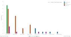
When manufacturing processes are under recipe control, the process moves to the next phase in a recipe when certain conditions are met. This is based on a timer, sensor reading, equipment or material availability, or another trigger. This typically produces a right-skewed distribution, where most of the data is close to the lower limit because small overruns are more common (Figure 1). As a result, the 25th and 50th percentiles are typically close together.
Using an automated approach, standard durations can be applied across all units. These durations are calculated for each batch phase over a reference time, and then applied to future results as lost-time benchmarks (Figure 2).
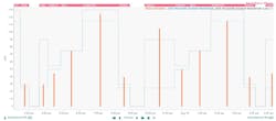
The 85th percentile identifies the worst delays for investigation. Also, there’s a second stipulation for classifying availability loss, occurring when phase duration is more than double the standard time, which keeps longer performance losses from being incorrectly labeled.
More complex logic could be used for assigning losses, such as classifying phases based on their dependencies, but this would require much more time to implement. For smaller operations and lower-value products, this wouldn’t provide a worthwhile return on the extra time invested.
Setting up the analysis
Beginning with start and end times for each batch phase, plus overall batch quality results, Syngenta employed Seeq to create its lost-time monitoring solution using the following approach:
1. Create an asset group to structure the data for production lines 1 and 2. This produces just one set of calculations to maintain, and it provides asset-scaling features to rapidly generate trends, comparative tables and reports for each asset of interest.
2. Calculate the actual duration of each batch phase.
a. Over a historical basis period, calculate the 25th and 85th percentile durations by phase.
b. Create 25th and 85th percentile benchmark signals that change with phase. This requires a key data analytics feature, where batch-phase, contextualized percentiles are spliced into one signal across time.
c. Join process batches to quality batches reported later, moving the quality result to the process operating period. This helps identify batch capsules, where the end-of-reaction test failed specification, which the advanced analytics solution does by linking time periods with matching batch ID, while retaining associated capsule properties.
3. Using one formula function, calculate a continuous signal for the accumulated time duration of each batch phase.
a. Search the signal for time periods when the duration goes above the 25th percentile benchmark. Create another search for time periods when the duration goes above the 85th percentile benchmark (and is also greater than twice the 25th percentile).
4. Using Seeq Value Search, Composite Condition, and time period manipulation functions, capture and quantify the lost time events.
a. Quality losses per batch = total batch duration for batches with a bad quality result.
b. For batches with good quality:
i. Availability losses per batch = sum (actual phase durations—25th percentile benchmark) for phases with duration > 85th percentile and duration > 2 x 25th percentile
ii. Performance losses per batch = sum (actual phase durations—25th percentile benchmark) for phases with duration > 25th percentile (and not an availability loss)
5. Calculate total productive time = total batch durations—availability losses—performance losses - quality losses
After creating each calculation step, Syngenta visually confirmed the result on the process trends (Figure 3) using Seeq Conditions with Capsule properties, and calculated metrics and signal values. Loss-category calculations were then combined with asset swapping and visualization options—such as histograms and tables—to analyze operational performance and find optimization opportunities.

Lost time monitoring and productivity insights
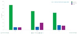
Lost-time monitoring results for a three-week period were analyzed in multiple ways. Reviewing time lost by phase (Figure 4) and loss type (Figure 5), the following insights were clear:
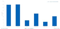
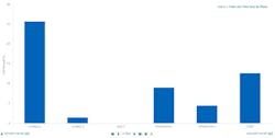
• The “react” phase is significantly worse on line 1 than 2. Investigation should look for differences in the “react” phase for both lines; and
• The largest loss category is availability. The biggest improvements can be obtained by reducing the wait time to start successive batches.
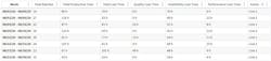
Examining the lost time splits in tabular form—and scaling the results across both lines (Table 1)—it’s apparent that line 2 is optimized compared to line 1, though both lines lose significant time each week. Line 2 usually produces more batches per week than line 1.
Increasing productivity using systematic analysis
In summary, modern data analytics were applied to batch manufacturing data at Syngenta to automatically classify lost productivity. By identifying delays, capable of scaling across a diverse range of production processes, the company took early steps toward increasing asset utilization.
After making process changes, lost productivity can be continuously monitored moving forward, demonstrating whether resultant changes achieve desired gains. Targeted and high-value improvement efforts are based on quantitative operations assessments.
In part two, we’ll explore how phase classifications in Seeq can be used to identify actionable root causes from process sensor data analysis. This requires considering correlations between multiple sensors, not just individual profiles.


Dr. Stephen Pearson is a principal data scientist at Syngenta. He helps worldwide manufacturing sites improve data management and analyses. John W. Cox is a principal analytics engineer at Seeq, where he works on advanced analytics use cases and provides technical input to new software features.
