Signal filtering: Why and how
Filtering is the modification of a measured or calculated signal—using an algorithm and/or logic—to remove undesirable aspects of the signal before it is used in a calculation or a controller. Examples in control are the feedback (or controlled) variable to a PID or APC controller, or the input to a feedforward controller. Calculation examples include computations based on steady-state material/energy balances or process-oriented relationships, as well as process and control metrics.
The main reason to filter a signal is to reduce and smooth out high-frequency noise associated with a measurement such as flow, pressure, level or temperature. A common example is the noise associated with the differential pressure (DP) across an orifice plate used to infer flow rate. High-frequency noise is normally considered to be random and additive to a measured signal, and is usually uncorrelated in time; i.e., the value of the noise at any time τ does not depend on previous values of the noise. Ideally, we want to estimate the underlying signal without noise, introducing as little distortion as possible.
When a noisy signal is used in control, filtering is important for effective derivative action and for avoiding excessive movement in the controller output that causes valve wear or disturbs other control loops. A complicating factor for the control case is that both filtering and controller tuning can be used to reduce movement of the controller output.
The problem of lag
The downside of filtering is the lag introduced, especially with heavier filtering, which can have a detrimental effect on timely detection of changes in the underlying signal. When used for feedback, the filtered value can result in control that is sluggish or, in the worst case, becomes oscillatory or even unstable. In the authors’ experience, the more typical problem encountered is excessive filtering of a signal, as opposed to under-filtering.
The source of the noise may be electronic or from the process itself. “Process noise” may originate from mixing, flashing, condensation/vaporization or from improper installation of a measurement device, for example, not enough straight-run pipe length upstream or downstream of a flowmeter. Unfortunately, in many cases, filtering is used in an attempt to mask the effect of an unmeasured disturbance or a problem such as valve resolution or dead band in the control loop. In many cases, the filtering makes problems worse. A filter will often be set and then forgotten until the loop is reexamined due to loop troubleshooting of poor performance, or when a control project is executed (e.g., APC).
Let’s consider the impact of filtering on PID loop performance. An important reason to filter the feedback variable (PV) is to ensure effective derivative action. Derivative action is important when aggressive control is required, particularly for integrating and near-integrating (lag-dominant) systems with additional lags(s) and dead time. If not properly filtered, noisy signals will cause derivative action to be ineffective due to erratic movement of the PID controller output. Fortunately, most industrial PID controllers include a filter on just the derivative term, expressed as a fraction, or divisor, of the specified derivative time. The fraction is usually in the range of 0.10 to 0.20 of the derivative time.
The other reason to filter the PV is to temper the controller output (CO) so the noise does not lead to excessive movement (and wear) of the valve, or cause disturbances to other control loops. In the past, another reason to filter the PV was due to resolution limits caused by the A/D converter, which would show up as noticeable steps in the measurement value; however, with 16 bit I/O cards, this is no longer an issue.
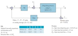
Figure 1: To evaluate filters in a closed loop, we simulate an integrating process with a noisy measurement signal and an aggressively tuned PID controller. Lambda tuning formulas modified by McMillan to provide better load disturbance rejection for a Standard Form PID (shown in Table 1) are used for an integrating process where seemingly insignificant noise is amplified by a high PID gain.
Simulation leads to optimization
To evaluate filters in a closed loop, we simulate an integrating system with a noisy disturbance signal and an aggressively tuned PID controller. The loop and simulation details are shown in Figure 1. Lambda tuning rules modified by McMillan to provide better load disturbance rejection for a Standard Form PID (shows in Table 1) were used for an integrating process. A value of λ = 2 sec (twice the loop dead time) was used as the arrest time (time to stop excursion) for the tuning, as it produced a non-oscillatory response in both the PV and CO, provided the system is linear and the dynamics are fixed and well known. The following loop criteria are evaluated for each filter:
Peak error: Maximum error following an unmeasured step in load. Peak error is important to prevent relief, alarm and SIS activation, and environmental violation.
IAE: Integrated absolute error over time is a common criterion for measuring loop performance. It directly relates to economics as it provides a measure of the amount of process material that is off-setpoint.
Setpoint overshoot: The maximum error overshoot for a setpoint change. Excessive overshoot can have economic or safety implications.
IAD: Integrated absolute difference of the controller output. For the case that the PID directly manipulates a valve, this is total valve travel distance and directly relates to valve wear.
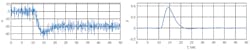
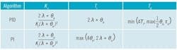
Figure 2: The closed-loop response in γ(process value before introduction of random noise) and μ(controller output) to a 20% step in load (d1 ) at time = 10 sec. for PID control without filtering clearly shows the effect of noise on μ.

For closed-loop evaluation of the filters, we decided to keep the PID tuning the same and not increase the filtering to an extent that causes cycling. Heavy filtering of the PV contributes lag and changes the process response, which would necessitate retuning. Since our objective is aggressive control, we want to minimize the impact of filtering on control, but reduce CO movement. Figure 2 shows the response in γ and μ (the CO) to a 20% step in load (d1) at time = 10 sec. for PID control without filtering. The effect of the noise on μ is clearly seen. Table 2 shows the results for PID control and, for comparison, also includes the results for PI control. While the PID achieves noticeably better PV results compared to PI, it does so at the expense of significantly more movement in μ.
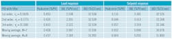
To evaluate the various filters for PID control, we tuned the filter parameter (ΤF or N) to achieve the same load IAD result (0.5423) as for PI control. Because the moving average parameter N is an integer value, it’s not possible to exactly match the same IAD value, so results are shown for filter N values above and below the PID value of 0.5423. Results are shown in Table 3 for both load and setpoint responses. We see that the first-order filter with PID control achieves worse results across all metrics than PI control with no filtering. Notably, the higher-order and moving average filters all perform better than PI control. The 2nd-order filter is the best performing filter across all metrics. Compared to the 1st-order filter, the 2nd-order filter achieves 7.3% smaller peak error and 19% smaller IAE for the load response, and 60% and 5.4% smaller peak error and IAE for the setpoint response. Compared to PID control with no filtering, the 2nd-order filter has 12% worse peak error and 3.9% worse IAE error for load response.
To compare all filters on exactly the same basis, we first select a moving average filter to achieve at least a 90% reduction in IAD compared to PID control without a filter; and then tune ΤF for the higher-order filters to achieve the same IAD. These results are shown in Table 4. Again, we see that the second-order filter yields better results across all metrics. Compared to the 1st-order filter, the 2nd-order filter yields 11% smaller peak error and 40% better IAE for load response, and 71% and 21% better results for the setpoint response.
Figure 3 shows the time responses for the 1st-order filter, and Figure 4 shows the time responses for the 2nd-order filter. The improvement from the 2nd-order filter over the 1st-order filter is clearly seen. Also seen in Figure 3 is that the response with the 1st-order filter is starting to become oscillatory. Note that at ΤF for the first-order filter, the loop becomes unstable. For the other filters, loop instability occurs at ΤF = 9.73 for the 2nd-order, ΤF = 0.45 for the 3rd-order filter, and N = 26 for the moving average filter. Thus it does not take much filtering to cause loop instability.
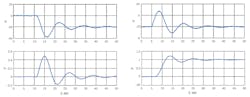
Figure 3: The PID closed-loop time responses for the load (left) and setpoint (right) start to become oscillatory and the loop becomes unstable at ΤF = 0.73.
Based on the above results, the closed-loop simulations show that significant improvement over the 1st-order filter is possible when significant noise is present, and aggressive control and significant reduction in IAD is needed. These results also show that a 2nd-order filter provides the best metrics, although not always by a large margin.
Conclusion: Don’t overdo it
What have we learned, what are the lessons? Be careful to not overly filter. What’s good to the eye is usually too much filtering, especially for control. Decreased attenuation of noise and disturbances comes at a cost: The more attenuation, the slower the filtered signal approaches a new average value—i.e., the more time lag. For the same amount of noise attenuation, higher-order filters (2nd- and 3rd-order) and the moving average filter approach a new average value quicker than the often-used exponential or 1st-order filter. The moving average filter can achieve higher levels of noise attenuation than the 2nd- and 3rd-order filters at the added cost of more coefficients and storage of previous signal values, but this should not pose a problem with today’s control systems. An advantage of the moving average filter is that it can eliminate a periodic cycle if the filter Δτ and N are selected appropriately.
When a noisy PV is used in control, the deciding issue to filter is unacceptable movement in the manipulated variable (controller output) caused by the noise. In this case, if aggressive control is required (higher gain with derivative action), higher-order and moving average filters allow tighter control with improved metrics (peak error and IAE) compared to the exponential or 1st-order filter.
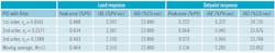
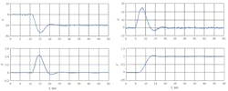
Figure 4: Comparing the PID closed-loop responses of a 1st-order filter (Figure 3) to the 2nd-order filter here shows improvements for both the load (left) and setpoint (right).
Before retuning a loop, make sure to note what the filter parameters are: time constant or filter factor and Δτ. Only use filtering to temper movement in the manipulated variable (controller output) caused by the noise. If aggressive control is required (higher gain and derivative action), higher-order and moving average filters allow tighter control with improved metrics (peak error and IAE) compared to the exponential or 1st-order filter. One should be careful to not cause loop instability with filtering. Although not extensive, these simulation results, plus others we have performed, generally show that of the filters considered, the 2nd-order filter provides the best metrics when targeting reduced levels of IAD.
We took the simple approach of keeping the tuning the same to show the improvement possible with more sophisticated filters. Ideally, the tuning and the selection of filter parameters should be jointly optimized, e.g., using a loop tuning optimizer.
Wait, there's more
We have focused on linear filters. However, the following additional suggestions are offered.
- When a process variable (PV) cannot respond faster than by an amount X/sec., a PV rate limit with this setting can be used to screen out noise without adding a lag. Alternatively, a setpoint rate limit can be put on the analog output block or secondary loop manipulated by the PID and external-reset feedback (e.g., dynamic reset limit) turned on to prevent the PID output from changing faster than the imposed setpoint rate limit. However, upon download or during tests for checkout and maintenance, the rate limit must be turned off.
- For pH measurements, the use of middle signal selection of three electrodes can reduce noise and eliminate spikes that commonly occur due to imperfect mixing and ground potentials without adding a lag, in addition to ignoring slower responding electrodes due to aging or fouling.
- For electrodes and temperature sensors, increasing back mixing and phase changes, and for pipeline installations, ensuring the tip is in the middle of the pipe at least 25 pipe diameters downstream of a pump discharge or equipment outlet can greatly reduce the source of process noise for these critical primary loops.
References
- Yang, W.Y. (2009). Signals and Systems with MATLAB. Elsevier, Inc., Oxford.
- Box, G.E.P., Jenkins, G.M., and Reinsel, G.C. (1994). Time Series Analysis, 3rd Ed. Prentice-Hall., Englewood, NJ.
- McMillan, G.K. (2015). Tuning and Control Loop Performance, 4th Ed. Momentum Press, New York.
About the Author

Greg McMillan
Columnist
Greg McMillan retired as a senior fellow at Solutia Inc., now a subsidiary of Eastman Chemical, in 2002. He was an adjunct professor in Washington University Saint Louis’ Chemical Engineering Department 2002-04, and retired as a principal senior software developer at Emerson Automation Solutions in 2024.
