There are several techniques that enhance PID controllers, termed advanced regulatory control. These were developed in the 1930s and 1940s, and include reset feedback to prevent windup, override to prevent excessive or unsafe conditions, and feedforward to correct an anticipated upset. Also, they include ratio, cascade, decouplers, gain scheduling, output characterization, and various forms of model-based adjustment. These techniques remain very useful today.
Ratio control bottom line
If you notice that one process variable should be a ratio of (proportional to, a fraction of, scaled to, or a similarly named relation) another influence variable (or to a calculated load or demand), consider ratio control. In ratio control, the output of the primary (supervisory) controller is the desired ratio, which is multiplied by the wild variable/demand/load value to become the setpoint for a secondary controller.
The wild variable is usually a flow rate, but it could be a compound variable calculated from material and energy balances such as a heat load. For example, the required steam flow rate to heat something to a target temperature depends on the process inflow rate as well as its temperature. The steam flow rate is proportional to the composite calculated value of the load,
Q? = F?C_p (T_SP-T_inflow).
The secondary (inner) loop needs to be faster than the primary loop for this method to offer an advantage. Some engineers use the rule, (?+3?)_secondary < ?1/5 (?+3?)?_primary.
Tune the secondary controller in the inner loop first, then tune the primary controller with the inner in AUTO. To the primary controller, the inner loop is just part of the process. If you tune the secondary after the primary, this changes the primary’s view of the process dynamics.
Ideally, you could calculate the ratio from first principles thinking, and not need the primary outer-loop controller. However, reality requires feedback from the primary controller to compensate for calibration errors of secondary sensors as well as unmodeled and non-ideal effects.
In ratio control, compensation happens as soon as the input change is detected, which is nearly as soon as the variable changes (given lags in sensors, controllers and valves). If the input change won’t affect the process for a while (perhaps because load calculations are based on far upstream measurements), then the ratio will cause compensation to happen too soon, creating an upset. If dynamic compensation is needed to match the timing of the control action to the process response to the disturbance, then use feedforward.
Blending example of ratio
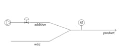
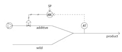
Figure 1 illustrates a blending process as an example. The wild flow is a process stream. The additive, which may be called a titrant, is added. The additive may be to adjust composition, pH or temperature, for example. Here it’s considered composition, and the analyzer transmitter (AT) measures and reports the mixed-stream composition.Figure 2 illustrates a primitive control strategy. If the reported composition is off-target, the analysis recording controller (ARC) adjusts the valve in the additive line to return the product to the correct composition. This primitive strategy works.
It‘s worth noting that, if the ARC were talking to the valve in English and using engineering units, it would be saying, “Valve, go to 53% open.” If the valve is air-to-open (fail-closed), abbreviated as ATO or FC, then the ARC needs to act in reverse. If the analysis of additive composition goes down, the controller output must increase to open the valve to compensate.Here’s a problem: if the wild flow rate increases, control action is delayed. The AT won’t detect the change until after the transport delay from the mix point to the sample point. Then, lags or delays in the AT won’t instantly report the full deviation. As the composition deviation is reported, the controller begins to respond, but the integral has a time-constant and will create a second lag. Finally, as the controller instructs the valve to change position, the valve will create an additional lag due to actuator dynamics. Eventually, the controller will return the composition to the setpoint, but not until the delay(s) and several dynamic lags have passed. During this time, there will be a persistent composition deviation.
Consider ratio. If the wild flow rate doubles, then the additive flow rate should also double. Rather than waiting for feedback correction, double the additive flow rate as soon as the new wild flow rate is detected.
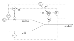
Figure 3 illustrates a ratio strategy. Here, the wild flow rate is measured, and the ARC determines a flow-rate ratio. This ratio multiplies the wild flow rate, which becomes the flow rate setpoint for the lower-level (secondary, inner) controller. The secondary controller is within a standard, flow-control loop.
The analyzer may be relatively noiseless, and the ARC may be PID. But the flow loop is probably a bit noisy and fast-acting, so the secondary should be PID.
It could be that the ARC isn’t in control for any number of reasons, such as the valve getting stuck or reaching a limit. FIC may be in manual. Instrument techs may have the valve on bypass. If so, the ARC will wind up to its limit of 0% or 100%. To keep its bias at the right value, use the actual flow rate ratio as an external reset feedback (ERF) signal.
The ratio strategy creates a role change for the ARC. The ARC is now talking to the multiplication block, and now it might be saying, “Hey, x-function, use 0.125 as the ratio.” The x-operation will also hear the wild FT say, “Hey, x-block, the wild flow rate is 220 gpm.” The x-block will multiply the two numbers, then tell the secondary flow controller, “Hey, FT, your setpoint is 27.5 gpm.”
In this case, the ARC continues to be reverse-acting. If the analysis value goes down, the ARC needs to increase its output, the ratio, to raise the flow rate setpoint to correct the deviation. In some ratio applications, the primary controller might change direction, for example, if the valve were air-to-close.The ERF signal must be the same as what the controller would be saying if it were in charge. It’s the actual flow rate ratio that might not be what the ARC wants (an operator could be adjusting the valve, the valve may be at a limit, the secondary controller could be in MAN mode). Use the lowest level transmitters in the control hierarchy to determine the ERF signal value.
There’s a strong similarity of the inner- and outer-loop structure between ratio and cascade. But the difference is that, in cascade, the primary controller sends a setpoint to the secondary controller. Meanwhile, in ratio, the primary sends a ratio to a multiplication operation, which sends the setpoint to the secondary.
Scaled signal calculations
If the signals and messaging between devices were to be in engineering units representing flow rates in gpm and temperatures in oF, it would be easy for a process engineer to understand the ratio strategy. But, of course, all these values are scaled values in the 0% to 100% range. As a result, the x-block needs to have an operation that keeps variable values consistent with the mechanistic meaning. For example, if the flow transmitter is scaled so that 0% to 100% matches the 0 to 500 gpm range, its output isn’t 220 gpm, but it is:
FT = (220-0) gpm /
(500-0) gpm (100-0)% = 44% (1)
If the ARC output is scaled so its full range of 0% to 100% matches a ratio range of 0 to 0.2, then its output is:
ARC = ((0.125-0) gpmA / gpmW) /
((0.2-0) gpmA / gpmW) (100-0)% = 62.5% (2)
The x-operation shouldn’t multiply 44% times 62.5%, obtaining 2,750%^2. What it must do is reconvert the 44% to the wild flow rate value and the 62.5% to the desired ratio, using the inverse of Equations (1) and (2).
Fwild = ((44-0)) / ((100-0)) (500-0) =
220 gpmW
Ratio = ((62.5-0)) / (100-0)) (0.2-0) = 0.125 gpmA / gpmW
Then multiply:
Product = 220 gpmW?0.125 gpmA / gpmW = 27.5 gpmA
Then convert the product to the 0-100% range that matches the additive flow range for the secondary controller. If this is 0 to 125 gpm, then:
xBlock = (27.5-0) gpmA / (125-0) gpmA (100-0)% = 22%
Similarly, the divide block needs to first convert scaled signals to their process units. So, do the division and convert the ratio to the appropriate scaled signal range for the ARC. If the wild flow rate is zero, then the divide operation will encounter an execution error. If so, it needs a calculation override, and a reportable default value, perhaps the last prior executable value.
If you choose ratio in your control devices, it might ask for the ranges and do the scaled signal conversions for you. But it might not.
Notes about Ratio
• The ratio control action happens immediately (as far as possible considering lags in sensors and final elements and delays in scan times) when the demand/load is detected. This prevents demand/load changes from upsetting the controlled variable.
• Ratio is easy to understand from a process engineer’s viewpoint, using values and units of the process variables. However, it probably needs to be implemented in scaled signal calculations.
• Relative to a primitive control strategy, ratio required two new flow transmitters and a new controller. The cost of installation and maintenance of these devices needs to be considered when the control benefit of adding ratio is being considered.
• The inner loop needs to be about five times faster than the outer loop for ratio to provide a substantial benefit.
• If the load is based on far upstream measurements, the delay in needing to change the additive may require a delay in the ratio implementation. Feedforward might be a better solution.
• ERF is not a requirement for ratio. It’s a complication to implement, and it may only solve a brief issue after some infrequent situations. I like it, but others may weigh the performance pros and implementation cons differently, and choose not to include ERF.
About the Author
R. Russell Rhinehart
Columnist
Russ Rhinehart started his career in the process industry. After 13 years and rising to engineering supervision, he transitioned to a 31-year academic career. Now “retired," he returns to coaching professionals through books, articles, short courses, and postings to his website at www.r3eda.com.


