Understanding the digital twin, part 1
“When I use a word, it means whatever I want it to mean.”
So began Louise Wright and Stuart Davidson in their recent article, “How to tell the difference between a model and a digital twin.”[1] Indeed, the words spoken by Lewis Carroll’s Humpty Dumpty in Alice’s Adventures through the Looking Glass might well be applied to any number of marketing campaigns discussing this latest, most fashionable moniker for a virtual representation of an actual phenomena. “Digital twin is currently a term applied in a wide variety of ways,” Wright and Davison continued, their message being that clarity of meaning is essential. Excessive marketing hype and one-upmanship name-dropping distorts a term, which leads to disillusionment about the concept, which leads to underutilization of a good thing.
This article is the first in a three-part series seeking to clarify what a digital twin means in the chemical process industries (CPI), how models and twins are used, and some techniques that can convert a model to a twin.
Model types
The term model also has many meanings. It could be a small-scale replica of an object used for dimensional analysis testing (such as for hull design of ships in a tow-tank) or entertainment (such as a train garden layout) or design (such as a tabletop replica of a chemical plant layout to visualize spatial relations). However, in the context of digital twins, the term model means a mathematical model that's been converted to digital code, which is used to mimic or simulate the response of the full-scale object. In the digital twin context, “full-scale” and “digital simulator” are key attributes for the model meaning.
We commonly use empirical, generic dynamic models in control, such as a first-order plus deadtime (FOPDT) model that's fit to process data to approximate the process response. These models are useful for tuning controllers and setting up feedforward and dynamic compensators. These and similar models (ARMA, SOPDT) have functional forms matching a predefined behavior. But just because we can get the model to comfortably approximate the process data doesn't mean the process behaves like the model. For instance, a high-order process with zero delay can be fit with a FOPDT model. That doesn't mean there's a delay in the process. In these cases, model coefficients don't have fidelity to the process, although they do have mechanistic meaning within the approximating model.
In a digital twin, model coefficients should represent a full-scale process attribute, such as equipment size, catalyst reactivity, valve characteristic, etc. There should be fidelity of the model coefficient to one property of the full-scale process.
We also use finite impulse response (FIR) models in model predictive control (MPC), neural-network models in soft sensors and inferential measurements, simple power-series (polynomial) models, and dimensionless variables in quantifying variable correlation. These are mathematically flexible models which don't express a predefined functionality.
Because of this, they're often termed “model-free” methods of representing a process. Many such approaches are in the toolkits associated with data analytics and machine learning. And again, although they're useful for discovering relationships, they don't seek mechanistic fidelity to the process. The coefficients in generic empirical models are adjusted to mimic what the data expresses, but coefficients in the model don't correspond to physical or chemical properties or dimensions of the process.
Contrasting empirical models, phenomenological (first-principles, mechanistic) models seek to express the human understanding of the cause-and-effect mechanisms of an object. They're based on material and energy balances, and use appropriate models of thermodynamic, kinetic, friction losses and other constitutive relations. Phenomenological models have mechanistic fidelity to the input/output (I/O) relations of the object, which permits them to extrapolate to new conditions. Coefficients in the model have a direct match to process sizes, object properties and behaviors. Phenomenological models are useful for exploring the impact of changes on the object properties and responses. Seeking fidelity of the model to the process, digital twins would prefer to use phenomenological, not generic empirical models.
In an extreme, rigorous phenomenological models seek perfection in representing every detail and nuance of the object with the most perfect of models. Although the ideal gas law may be fully functional for use in a particular model, a rigorous “show-off” approach might be to include the Benedict-Web-Rubin-Stirling or a Virial Equation of State, just because it's most advanced. Tempering a sense of ultimate scientific perfection, the fidelity sought in a practicable model should be appropriate to the functional use of the model in the given application.
This means that, instead of using the partial differential equation that would be the “right” way to model the distributed temperature of fluid in a heat exchanger, the modeler could choose to approximate that truth with a FOPDT model in which time-constant and delay values are mechanistically scaled to flow rate. The inclusion of some empirical models may be pragmatic.
Although phenomenological models are preferred, the models desired in a digital twin will seek to balance perfection with sufficiency, to have fidelity to the requirements of the application that use the model, not necessarily to represent an ultimate in modeling perfection.
An object of the model
The “object” being modeled could be a mechanical device, chemical process, electronic device, building, distribution system, aircraft, communication system, etc. Although the object could be a single control valve, it could also be all devices within that control loop (current-to-pressure, or i/p, wireless connection, actuator, etc.) including their features (stiction, digital discrimination, dropped messages, etc). The object could also be the heat exchanger, including its associated instrument system, or the distillation column with that heat exchanger, or the separation process unit containing the column, as well as tanks and startup and safety items, or some larger assembly. The object doesn't need to be a single entity; it could be the composite of many interacting objects.
The object can also be a batch or continuous process.
Model uses
The use of models isn't new in the CPIs. Simulators using mathematical models of objects are essential for design, fault detection, performance analysis, knowledge development, process improvement, training, process optimization and many other human initiatives. Phenomenological models can be used in model predictive control and as inferential measurements. When the engineering and operational staff understand the process through phenomenological models, they'll better understand cause-and-effect relations, and be better at troubleshooting and process improvement.
The rationale to use phenomenological models (and digital twins) is to actualize all those potential benefits.
What’s new about twins?
Digital twins are simulators based on models. So what makes them different from a model-based simulator?
Following the guide of Wright and Davidsont, the digital twin of an object entails:
- a phenomenologically-grounded digital simulator of the full-scale object,
- an evolving set of data relating to the object, and
- a means of frequently updating or adjusting the model in accordance with the data.
We're familiar with Item 1, simulators based on phenomenological models of the full-scale object. We commonly use both text-book type models of units and software providers’ simulation packages for process design and many other modeling applications.
Item 1 is a model. Items 2 and 3 differentiate a model from a twin.
Item 2 represents data from the real world that's used to adapt, adjust or update the model. In chemical processes, this data could be related to reconfiguration changes, such as piping paths, taking a parallel unit offline for maintenance, shifting a raw material supply source that changes its character, lowering tank levels to meet end-of-year inventory desires, and others. The data from the process could also relate to attributes that change in time, such as catalyst reactivity, heat transfer fouling, tray efficiency, or fluid friction losses in a pipe system. The data is called an evolving data set, meaning data is continually (or at least frequently) acquired, and reflects properties of the object that are ever-changing.
Item 3 indicates that the model is adapted to retain fidelity to the real object. “Frequently updating” means the model is continually updated (or at least frequently enough to keep the twin locally true to the object). This could mean model objects are rearranged to match process reconfigurations, that model constituency relations are changed to best match the data (the ideal gas law could be replaced with a Van der Waals model if data shows it should), or that model coefficient values are adjusted to make the models best match the data (such as product yield, tray efficiency or inline flow restriction).
This digital twin concept already is familiar in the CPIs. It's not uncommon to “calibrate” phenomenological models or process simulators, so they match the actual process behaviors. Then the models can better represent constrained conditions, operating possibility, optimum setpoints and KPIs in general. Calibrated models are more accurate. If you calibrate simulators with recent plant data, then you're creating digital twins.
Outside the CPIs, in manufactured products (compressors, refrigeration units, cell phones, cars, etc), the in-use data from an object can be related to conditions of use and degradation of that object. The Internet of Things (IoT), in turn, can provide real-time access to data from onboard sensors. The twin is then a common phenomenological model that's adjusted with data from the object, and can be used for situation monitoring.
For the chemical process operator, access to data from the process has long been available through local area networks (LAN) and digital control systems. Here, digital twinning, recalibration of models to match the process, is no longer a groundbreaking concept. However, for manufactured products, access to onboard data from remote objects is relatively new. The concept of a digital twin may be more newsworthy in that context.
Classically, however, chemical plants were built with the minimum investment in instrumentation necessary to effect adequate safety and control. To achieve a true digital twin, more sensors, sensors with greater precision, and techniques for data validation (such as voting, data reconciliation and inferential sensors) will likely be needed to permit valid model recalibration.
Process simulators and control
Simulators for chemical process design use steady-state models of continuous process units, or end-of-batch models, and are fully adequate for many design, optimization and analysis purposes. Increasingly, simulation software providers are offering dynamic simulators of process units that include emulations of controllers. These can be very helpful in exploring the transient behaviors in response to startup, transitions and disturbances. However, as McMillan, et al.[2] point out, the controllers provided in process simulations are often primitive. The process simulators may not include advanced regulatory control options, nonlinear characteristics of installed valves, or data processing features and digitization characteristics of a controller. Those authors suggest that a digital twin should include dynamics, controllers, and any structure of the control system that might affect I/O relations. Preferentially, a dynamic simulator of the object would be connected to either a real controller or a twin of it to have the control aspects represented in the digital twin of the combined process-controller system.
Twin functionality
The intended use of a digital twin (or a model) will define essential properties that the model needs to express. For instance, if the digital twin is going to be used for supervisory setpoint economic optimization or scheduling, then steady state models that adapt to process characteristics and associated operational constraints may be fully adequate.
However, if the purpose is to explore or tune control strategies, the models of sub-objects should include their dynamic response. Further, to test control strategies and to quantify goodness of control metrics, stochastic (ever-changing) inputs to the model should include the vagaries of environmental disturbances (such as ambient conditions and raw material variation), operational uncertainties (such as mixed-feed compositions, instrument noise, reactivity, fouling and other process attributes that change in time). These stochastic inputs can be created with auto-regressive moving-average (ARMA) models that mimic the real-world experience of both the variability and persistence[3]. These models could then be used to define setpoint values that are comfortably away from specifications, so that variation doesn't create safety or product violations.
Generating stochastic input values
A recommended way to generate stochastic inputs is to consider that they're first-order responses to disturbances. In Equation (1), the variable x represents the first-order influence on a process from a disturbance d, with a first-order time constant of τ:

Analytically, the solution can be converted to an incrementally updated new time sample by Euler’s explicit method.
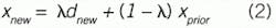

Here, Δt is the simulation time step, or sample-to-sample time interval. If the influence, d, is not a constant, but continually changes, then the new x-value is influenced by the new d-value.
If dnew is modeled as randomly changing in a Gaussian manner with a mean of 0, and variance of σd, then it can be modeled using the Box-Muller[4] formula:

where r1 and r2 are independent random numbers uniformly distributed on an interval from 0 to 1 (your standard random number generator). Then, the first-order persistence driven by NID(0,σ) noise and averaging about a value of xbase can be is modeled as:

In creating a simulation with a stochastic influence, the user would choose a time-constant for the persistence that is reasonable for the effects considered, and a σx-value that would make the disturbance have a reasonable variability. At each sampling, Equation (5) would provide that stochastic value for the variable x. The stochastic variable could represent barometric pressure, ambient heat load, raw material composition, or any such ever-changing influence or process character. In its first use, the value for xprior in Equation (5) should be initialized with a characteristic value, such as xbase.
How should one choose values for λ and σd? First consider the time-constant, τ, in Equation (1). It represents the time-constant of the persistence of a particular influence. Roughly, τ ≈ 1/3 of the lifetime of a persisting event (because the solution to the first-order differential equation indicates that after 3 time-constants, x has finished 95% of its change toward d). So, if you considered that the shadow of a cloud persists for 6 minutes, then the time-constant value is about 2 minutes. Once you choose a τ-value that matches your experience with nature, and decide a time interval for the numerical simulation, Δt, λ calculate from Equation (3).
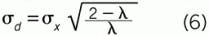
To determine the value for σd, propagate variance in Equation (5). The result is Equation (6). Use your choice of σx (and λ, which is dependent on your choices for Δt and τ) to determine the value for σd:
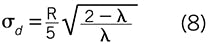
Choose a value for σx, the resulting variability on the x-variable. To do this, choose a range of fluctuation of the disturbance. You should have a feel for what is reasonable to expect for the situation you're simulating. For instance, if it's barometric pressure, the normal local range of low to high might be 29 to 31 inches of mercury; if outside temperature in the summer, it might be from 70 to 95 °F; or if catalyst activity coefficient, it might be from 0.50 to 0.85. The disturbance value is expected to wander within those extremes. Using the range, R, as
R = HIGH – LOW (7)
And the standard deviation, σx, as approximately one-fifth of the range, then
As a summary, to generate stochastic inputs for dynamic simulators, choose a time constant for persistence of events and a range of the disturbance variable. Use Equation (3) to calculate λ, then Equation (8) to calculate σd. Then, at each simulation time interval, use Equation (5) to determine the stochastic input.
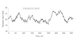
Figure 1 is an illustration of one 400-min realization of a stochastic variable calculated as above. The time-constant is 40 min, the nominal value is 20, and the range is 3 units. In this one illustration, notice that the variable averages about its nominal value of 20, and the difference between the high and low values is nearly 3. From a period between 150 and 275, the value is below the average, indicating a persistence of 275 -150=125 min, which is about three times the 40 min time-constant. Some persistence values are shorter, some longer.
Key takeaways
A digital twin is a simulator that is frequently calibrated with data from its object. Preferentially, the models in the simulator are phenomenological. The twin seeks adequate fidelity to the aspects of the object that are functionally important. It doesn't seek perfection in what it uses for constituent relations, nor to model aspects that are irrelevant to the application utility of the simulator.
Having a digital twin permits offline exploration of design changes, structuring controllers, economic optimization within constrained conditions, hazard analysis, predictive maintenance, training, and many applications.
Using frequently recalibrated models may be nothing new to you as a process operator. But for some, especially related to manufactured products, the concept of twinning each individual object in use, from its individual data, for individual analysis seems to be relatively new. Such applications may be shaping the news.
Effective twinning in the CPIs may require additional process instrumentation and data verification and correction techniques to have the valid feedback needed to recalibrate models.
The model type, the features in the model should be appropriate to the model use. If, for instance, to test controllers, the twin should include the vagaries of input and ambient disturbances, equipment attributes and operational conditions.
[This article consists of three parts. Parts 2 and 3 of this series will be published in the November and December 2021 issues of Control. This first part was on the utility of using models, what sort of models there could be, benefits and disadvantages for them when used as a digital twin. The second part will discuss methods for both initial and on-line model adaptation. And the third part will be about tempering the adaptation of the model coefficients when in response to noise and spurious signals.]
References
- Wright, L., Davidson, S. “How to tell the difference between a model and a digital twin”, Adv. Model. and Simul. in Eng. Sci. 7, 13 (2020). https://doi.org/10.1186/s40323-020-00147-4.
- McMillan, G. K., C. Stuart, R. Fazeem, Z. Sample, and T. Schieffer, New Directions in Bioprocess Modeling and Control, 2nd Edition, ISA, Research Triangle Park, N.C., (2021).
- Rhinehart, R. R., Nonlinear Regression Modeling for Engineering Applications: Modeling, Model Validation, and Enabling Design of Experiments, Wiley, New York, N.Y., (2016).
- Box, G. E. P., and M. E. Muller, "A Note on the Generation of Random Normal Deviates," The Annals of Mathematical Statistics 29 (2): 610–611, (1958).
About the author
Russ Rhinehart started his career in the process industry. After 13 years and rising to engineering supervision, he transferred to a 31-year academic career. Now “retired,” he enjoys coaching professionals through books, articles, short courses and postings at his website www.r3eda.com.
About the Author

R. Russell Rhinehart
Columnist
Russ Rhinehart started his career in the process industry. After 13 years and rising to engineering supervision, he transitioned to a 31-year academic career. Now “retired," he returns to coaching professionals through books, articles, short courses, and postings to his website at www.r3eda.com.
