Understanding the digital twin, part 2

The digital twin begins life as a prototype model, intended to match the process, but possessing ideal attributes that need to be adapted to the actual process. First, one must adjust model coefficients and constituent relations to best match the model to actual process operation. Second, over time as the process is reconfigured or substantially altered, reflect those process changes in the model. This may also require adjustment of model coefficients. Third, as the process operates, there will be continual changes in features such as ambient heat losses, heat exchanger fouling, catalyst reactivity, friction losses in piping, raw material properties, etc. Incrementally adapt the model to match the local reality.
This is part 2 of a three-part series on the digital twin. Part 1, in the October issue, defined a digital twin as a model of the process that's frequently adapted to match data from the process. This keeps it useful for its intended purpose. Here, part 2 discusses how to adapt the model. And part 3, in the December issue, will discuss tempering adaptation in response to noise.
Do not attempt to code the entire composite model at once. Make the model modular. Construct each elementary object as its own model, coded as its own subroutine or function block. Use its output as the input for another sequential object module. Build the process digital twin as a collection of interconnected subroutines. This permits the individual models to be easily adapted with limited data, to be edited, and to be understood.
Adjust coefficients and relationships
Begin by adjusting the component models individually. There are two aspects to this adjustment step: 1) changing internal models and 2) adapting model coefficient values. The first stage is to change internal models that are not quite right. For example, the model may have been initially developed with an ideal Bernoulli square-root relationship for friction losses in a line, but data might indicate that a power law gives a better representation. A reactor may have been initially modeled as an ideal plug flow device, but data might reveal that a series of continuously stirred tanks (CST) might be a better model. A reaction may have been modeled with an ideal homogeneous model, but process data might suggest that a mass transfer limited kinetic model is better. Change the modeled functionalities to match the process behavior.
The second stage is to adjust model coefficient values to make the model best fit the data. Many model coefficient values have high uncertainty (friction factors, reactivity, yield, ambient losses) which also change in time as the process is used. Here, classic least squares minimization of the model-to-process data difference (the residual) is justified. This would probably be a nonlinear optimization [1]; and although it could be automated, often human intuition and choices regarding which model coefficients should be changed, and which sections of the data are most important, might make human-guided model adjustment more appropriate than sophisticated algorithms.
Normal historical operating data might have enough information to permit such adjustment, but historian data will probably not have the richness required, and some purposeful input changes may be needed to get the required data. Further, old historical data could very well represent equipment and procedures that are no longer in practice. Such data should not be used to create a twin of current practice, so be prepared to not respect the treasured historian database.
Over time, the process will be reconfigured or substantially altered. Piping paths will be rerouted. Old units will be replaced with not-quite identical ones. Five units operating in parallel will be reduced to four when one is taken offline for upgrading. Reflect those changes in the model. This may also require re-adjustment of model coefficients.
Incrementally update the model
The prior model adaptations can be considered as one-time changes in response to a batch of data. However, as the process operates, there will be continual changes in ambient heat losses, heat exchanger fouling, catalyst reactivity, friction losses in piping, raw material properties, distillation tray efficiency, etc. Use process data to incrementally adapt the model to match the local reality
The processes might be classified as either continuous or batch. However, as they operate in time, attributes change in time, and values for those attributes are needed for analysis or control.
In such cases, the coefficient of interest changes in time. If one were to collect all historical data for regression, earlier data would express one value of the time-changing coefficient, and recent data will express a different value. Rather than adjusting a model on old data, and reflect an outdated property value, models are often incrementally adjusted to match the most recent data.
Process features or attributes that change with time, require the model coefficient values to change in time. Such models are termed non-stationary. Process owners observe that the model coefficient values that reflect such factors to inferentially monitor process condition, performance or health, and use that information to trigger events, schedule maintenance, predict operating constraints, and bottleneck capacity, etc.
The choice of which model coefficient is to be adjusted should be compatible with the following five principles:
- The model coefficient must represent a process feature of uncertain value. (If the value could be known or otherwise calculated, incremental adjustment wouldn't be needed.)
- The process feature must change in time. (If it didn't change in time, adaptation would be unnecessary.)
- The model coefficient value must have a significant impact on the modeled input-output relation. (If it has an inconsequential impact, there's no justification to adjust it.)
- The model coefficient should have a steady-state impact if data are to come from steady-state periods. (If it doesn't, if for instance the coefficient is a time-constant, then when the process is at, or nearly at, a steady-state, the model coefficient value will be irrationally adjusted in response to process noise. Since continuous processes mostly operate at steady conditions, this is important.)
- Each coefficient to be adjusted needs an independent response variable.
If one or more of the five principles aren't true, there's no sense in adapting that model coefficient online.
There are many ways to update model coefficient values, to adapt models in real-time, which have led to a variety of adaptive control methods. If you're lucky, you'll be able to rearrange the model equation and explicitly calculate the model coefficient value from data. However, you might not be able to do that for any of many reasons, one being that the model is calculated from a procedure hidden in a function. What follows is a summary from a simple and effective approach to incremental adjustment of a phenomenological model [1].
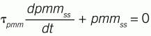
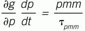
The desire is to adjust a model coefficient representing steady-state response, so the process-to-model mismatch (pmm) approaches zero in a first-order manner when the process is near steady conditions. The mathematical statement of that desire is:
(1)
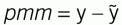
Where:
(2)
Representing the steady state process as:
(3)
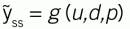
in which ỹ is the modeled response and ỹss is the steady-state modeled response, u is the modeled controller influence on the process, d represents measurable disturbances, and p represents the coefficient that will be incrementally adjusted.
As indicated, equation (3) might be an explicit equation. More likely, it will be calculated as a procedure (function or subroutine) and the result will be a numerical value for ỹss.
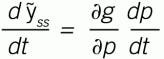
If p, the coefficient value changes, then ỹss will change. If near to a steady-state condition, the y, d and u values are not changing. Then, using the calculus chain rule on Equation (3), the change in ỹss with respect to time is:
(4)
Substituting Equation (4) into (1) and rearranging:
(5)
Rearranging for incremental model coefficient adjustment using a simple numerical solution (Euler’s explicit finite difference):
(6)
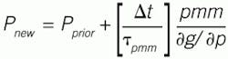
Equation (6) is a Newton’s method of incremental, recursive coefficient updating (root finding), with the bracketed term as a tempering factor. The user’s choice of the value of τpmm prevents excessive changes in the model coefficient value and tempers measurement noise effects. The sampling interval, ∆t, has the same time units as the time-constant, and provides a normalizing factor for the frequency that the model is updated.
In computer assignment statements, the subscripts new and prior are unnecessary because the past values are used to assign the new value.
The value of τpmm should be large compared to model dynamics (so that model adjustment doesn't interact with control calculations), but small compared to the time period over which the process attribute changes (for rapid tracking of the process).
Don’t let the derivative representation be off-putting. It just means sensitivity. And it doesn't require calculus. It can be easily evaluated numerically. The term [ ∂g/ ∂p] means the sensitivity of the modeled steady state response, ỹss, to the value of the adjustable coefficient, p. You could calculate the sensitivity numerically as:
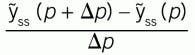
This can be calculated from equations, if you have them, or from using the subroutine procedure to calculate the ỹss values for two p-values.
Example calculations
As a relatively simple process example, consider the overall heat transfer coefficient on an ideal counterflow heat exchanger using first-principles, constitutive models. The steady state design equation is [2]:
(7)

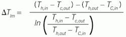
Here, Q̇ is the rate of heat exchanged, UA∆Tlm is the model for heat transfer, U is the overall heat transfer coefficient (which will change in time with fouling), A is the heat transfer area, and ∆Tlm is termed delta-T-log-mean, representing the characteristic temperature driving force for heat transfer. The heat transferred is the same as the heat picked up by the cold fluid, FcρcCpc∆Tc with ∆Tc = (Tc,out – Tc,in) and that lost by the hot fluid, FhρhCph∆Th with ∆Th =(Th,in – Th,out).
Given inputs to the heat exchanger and heat exchanger properties, U and A, the model can be used to calculate the two outcomes Tc,out and Th,out. I haven't figured how to get an explicit arrangement, so I use a trial-and-error procedure: Guess at the value of Tc,out , use the relation FcρcCpc∆Tc = FhρhCph∆Th to solve for an associated value for Th,out, then search for a Tc,out value that makes UA∆Tlm = FcρcCpc∆Tc. Although represented by the single Equation (3), calculating Tc,out from the inputs is a procedure, not a single line equation.
The overall heat transfer coefficient will change in time with fouling. In Equation (7), the variable p represents U in the example, and ỹss represents Tc, out. The required sensitivity in Equation (7), is the sensitivity of Tc,out to U and will be calculated numerically by comparing the calculated value of Tc,out with two U-values [Tc,out(U+∆U) – Tc,out(U)]/∆U].
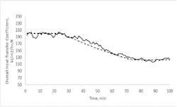
Figure 1: Illustration of using process data to incrementally update a model coefficient.
Figure 1 indicates how the incremental updating of the Twin coefficient tracks the process value. In a simulation, we can know the true value of U, which is represented by the dashed line that starts at a value of about 200, then ramps down to a value of about 130. During this simulation, inlet flow rates and temperatures are continually changing, and there's also noise on all measured values. The solid line in the figure represents the Equation (6) procedure to incrementally update the model U, with a τpmm = 3 minutes. It tracks the actual very well. The variation in the estimated value of U is due to the measurement noise on the flow rates and also on the temperatures.
One benefit of this procedure is monitoring critical process attributes, such as a heat transfer coefficient, possibly to be able to schedule maintenance.
Another benefit is to be able to forecast constrained operations, which is illustrated in Figure 2, for the same period simulated in Figure 1. In Figure 2, the twin is asked, “What's the possible outlet temperature for the fluid being heated given the maximum heating conditions and a target process fluid flow rate?” With the clean heat exchanger, this estimate fluctuates at about 324K, but as fouling happens, the maximum achievable temperature drops to about 308K. Alternately, the twin could be asked, “What's the maximum process flow rate for which the heat exchanger could maintain a setpoint temperature?” This forecast of constrained conditions would be useful for supervisory optimization and planning.
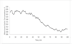
Figure 2: Illustration of predicting constrained operating ability.
To keep a model true to the process, to create a digital twin, start with the prototype models as a collection of sub models. Collect data to compare model to process. Adjust model equations to best match actual process phenomena. Adjust model coefficient values to best match models to process data. Reconfigure the models anytime the process is reconfigured. Continually adapt the model coefficients in time as process characteristics drift.
The legitimacy of process analysis using models depends on the fidelity of the model to the actual process behavior.
It takes a lot of work to nurture twins.
References
[1] Rhinehart, R. R., Nonlinear Regression Modeling for Engineering Applications: Modeling, Model Validation, and Enabling Design of Experiments, Wiley, New York, NY (2016).
[2] Incropera, F. P., and D. P. De Witt, Introduction to Heat Transfer, Wiley, New York, N.Y. (1985).

About the Author

R. Russell Rhinehart
Columnist
Russ Rhinehart started his career in the process industry. After 13 years and rising to engineering supervision, he transitioned to a 31-year academic career. Now “retired," he returns to coaching professionals through books, articles, short courses, and postings to his website at www.r3eda.com.
