Data integrity series: Digital degradation in data path

This is the second in a series of discussions with Mike Glass, owner of Orion Technical Solutions, on ensuring data integrity for process control and industrial automation systems. Orion specializes in instrumentation and automation training and skills assessments. Glass holds ISA-certified Automation Professional (CAP) and Certified Control Systems Technician Level III (CCST III) credentials, and has nearly 40 years of I&C experience across multiple industries. 

Greg: We previously talked about how filtering and damping help clean up the raw analog signal before it’s digitized. Let’s continue following that signal downstream. What happens once it becomes digital data and starts moving through the system?

Mike: Once a signal leaves the analog world, a new set of data-degradation issues appear.
Digital precision, timing and synchronization become critical, and if we aren’t careful, they can quietly distort what the controller and analytics see.

Even after the input has been sampled in the analog input card, there are several points in the data path where errors can be introduced or magnified—through data timing variability, scaling mistakes, rounding, bit-depth losses or historian compression. Many of these occur at multiple points along the signal path, and their effects can build up until the data no longer represents the real process.

Greg: What types of problems do you see when it comes to timing and synchronization? 

Mike: Network latency, jitter and misaligned time stamps are some of the first significant contributors to digital degradation. Even small timing variations can cause controllers to interpret signal changes incorrectly.

Inconsistent data intervals—or jitter—can make the process variable appear to change at rates that are different from reality. This is especially problematic for high-gain PID loops, derivative actions or processes with exponential characteristics. You can see this illustrated in the signal flow diagram below. 

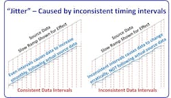
Even if the raw signal was clean and perfectly accurate, timing irregularities can cause the data to inaccurately represent rates of change. It can cause inaccurate data for specific time intervals since the data may have been slightly above or below the actual value it would have been at for a consistent data interval sample. 

Greg: What are common causes you have seen for this type of error? 

Mike: Asynchronous data transfers are the biggest causes of these errors. If the sampling, communications and storage of data aren’t intentionally lined up and organized, the data records no longer represent a specific point in time—and jitter is introduced. From there, it’s often magnified due to additional steps of inconsistent timing/sampling throughout the system. To prevent these problems, great care must be taken to ensure that the sampling, update and comms timing is consistent and synchronous. 

The best solution for this problem is to use time-stamped data systems. Time stamps help solve many problems in the digital data path, but they add cost for the sampling modules and for storing additional data. 

Greg: What problems or issues have you observed with time-stamped systems? 

Mike: Controllers, PLCs and historians use independent internal clocks or clocks that aren’t routinely aligned. Even small drifts—a few milliseconds per day—can cause problems when analyzing time-based events and trends. 

Greg: Can you give an example?

Mike: One offshore oil production platform I worked on had a wide mix of vendor-based systems providing their own data and often their own time stamps. Some weren’t even time-stamped, so the system assigned a time stamp when the data arrived—often many hundreds or thousands of milliseconds later. 

When a turbine or compressor tripped, the resulting transients and impacts caused a cascade of other events and trips along with subsequent high vibration, pressure, flow and other alarms and trips within milliseconds of each other. The mismatch of time-stamp data made it very difficult to definitively determine actual root causes of problems in many cases.

Imagine a super-intelligent system analyzing that same data and looking for relationships and causes without realizing the data-timing isn’t asynchronized From experience and other system networking and comms details, we lowly humans knew the typical time lags and factors that would affect them, so we could often see through the misleading data time stamps However, a typical machine or intelligent system may not be trained to see that level of detail, and could easily see the hatchling chicken before the egg, resulting in faulty analyses and errant results. 

Greg: That’s a great example of why accurate and synchronized time stamping is important. What other examples do you have where the timing becomes critical? 

Mike: When evaluating a system’s control performance, looking back at control valve position vs. command position, setpoint, manual output percentage and various load factors can be an incredibly powerful tool. If the data isn’t accurately represented by a synchronized time stamp, the relationships become disconnected, and it becomes much less useful or could even be misleading. Any time-based analysis needs accurate, synchronized timing. 

Greg: Mismatched time stamps are a problem. What solutions have you seen for it?

Mike: The best practice is to use GPS-synchronized clocks or precision/network time protocols (PTP/NTP). Modern GPS modules can provide accurate universal time references directly into control networks. This ensures every device—from transmitters to servers—shares the same timeline, eliminating those small but misleading offsets. Modern GPS time servers typically cost less than a typical analog input. If that’s not an option, at least ensure that all devices that must be analyzed are time-stamped, and are regularly synchronized to minimize deviations.

Greg: Let’s move to math and scaling. I know you’ve seen rounding and integer math cause hidden troubles.

Mike: Yes, one of the most common and easily preventable problems is excessive or assumptive rounding. Simplified constants like using 14.7 psi instead of 14.6959 psi for atmosphere, or dropping the 0.15 from 273.15 K, add small but cumulative offsets. Over multiple conversions, that rounding can bias calculations or energy balances.

Greg: What about integer math issues? 

Mike: One of the big minefields in the data path is integer math, especially in older or auxiliary systems that still use integer registers for analog scaling or totals. 

There are a ton of these integer-based systems in the data path, more than many assume. Many are overlooked, and it’s assumed they’ll operate like high-bit, floating-point-type systems. It’s wise for control engineers to audit the major data paths of critical systems to ensure they’re “eyes open” to potential problems that are often overlooked. 

Integer math only handles whole numbers. This means:

• Truncation — Integer division drops remainders (7 ÷ 2 = 3, and even less intuitively 1 ÷ 2 = 0 and 3 ÷ 2 = 1). The remainders are truncated (omitted), not rounded. Great care must be exercised when programming any math in the controller when using integers. As a rule, scale up the numerator when doing integer math. You’ll often see multipliers of 1,000 on the numerator, and then division by 1,000 to obtain the final answer. So, in our example, 7 ÷ 2 = 3; we enter 1,000 x 7 = N1; then we calculate N1 ÷ 2 =  (7,000 ÷ 2) = 3,500 = N2; and we use the scaled value of N2 in HMI and other calculations. But, we must also be cautious of overflows.
• Overflow — When a calculation exceeds the integer’s range (+32 767 for 16-bit, +2 147 483 647 for 32-bit), it wraps negative. Totals or logic can suddenly reverse or zero without warning. In many systems, this can result in major faults that will halt the processor and cause system shutdown. Integers are a headache anytime we really want decimal values, so the optimal solution is to just use real (floating-point) number systems when possible. 
• Cumulative loss — Small truncations repeated thousands of times (e.g., in totalizers) create measurable drift. It’s important to remember that the remainders are omitted, not rounded when using integers. Adding 1.5 + 1.5 + 1.5 + 1.5 would essentially be like adding 1 + 1 + 1 + 1, so the total would be 4 instead of 6. 

Greg: Those integers can indeed cause problems. What advice do you have for anyone who has some of those integer-based systems in their data stream path?

Mike: 

1. Multiply before dividing to keep numbers larger, so fractional accuracy is longer. Be careful not to cause overflow results. It can be a tricky compromise finding the balance between potential overflow results and adequate resolution. One must always remember that real analog inputs can possibly go a little beyond the assumed 0-100% range as well.
2. Use wider intermediates like DINT (32-bit) or 64-bit if available since they’ll have a larger range of base values and provide more resolution.
3. Monitor overflow bits and clamp results. In some cases, it’s also wise to set up fault routines that will catch, manage/resolve, report, and possibly automatically reset certain overflow errors.
4. Move critical scaling to floating-point (REAL) whenever possible.

Most modern PLCs and DCS handle floating-point values efficiently, and float precision (≈ 1 in 8 million) is a small fraction of typical transmitter errors and noise. You’ll still find those integer-based systems on many small, interconnected, mini- and micro-controllers, and various systems that are often provided as utilities or auxiliary equipment, such as compressors, GTs and more. Use integers for counters and discrete logic, but for analog math, floating point is the way to go if possible. 

Greg: What other math-oriented problems have you seen cause problems in the data stream?

Mike: Sometimes the gain or the magnitude of an error seems more dramatic in certain situations. A good example of this would be DP Flow. At low flows, a small DP error, which is common, can cause a significant apparent error in flow value. As the flow increases, the slope of the transfer curve increases, so the DP error is attenuated. 

Of course, in the field, we typically don’t rely on DP-based flow measurements for low-in-range control or readings (below 50%), but sometimes the intelligent systems and/or operators may not realize it. Or, they may not understand the concepts of DP flow, and may be confused by a -10% error when the pump is off, and they know the flow should be 0%. Of course, that error rapidly reduces as we ramp up to normal operating flow ranges. There are many situations where the impact of errors varies considerably through the operating range or through various process conditions, and these need to be carefully factored into any data analysis. A savvy controls professional can identify most of these types of issues to help improve accuracy of analysis and findings. 

Greg: You mentioned the issue of bit-depth resolution. What do you mean by that?

Mike: Bit resolution is less of a problem today than it once was because systems are now typically 16-bit or higher. But there are situations where 12-bit data is used along the data path—sometimes without the engineers fully realizing it. 

When a high-resolution device—a 24-bit scale—feeds a 16-bit input card, those extra eight bits of resolution are lost forever. That’s like taking a 16-million-step measurement, and rounding it down to 65,000 steps. The table below contrasts some common bit-depth values. 

Source: Orion Technical Solutions

Greg: What are your thoughts on required bit-depth for most equipment? 

Mike: For most process systems, where a 0.1% value is totally acceptable, if a system is in the 16-bit resolution range or more, we rarely notice any problems. If an input comes from a 12-bit analog input, for example, or if much higher precision is required, a low-resolution bit depth can become a problem.

The resolution of a 32-bit floating point number is approximately 1 in 8 million across most of its range, but its ability to do complex calculations without any trickery is even more helpful. When floating point numbering was implemented in early control systems it changed the game, and paved the way for process control capabilities. 

Get your subscription to Control's tri-weekly newsletter.

Greg: It’s remarkable how often clean data isn’t clean at all. By the time it reaches the historian, it’s been filtered, compressed or averaged half dozen times. Smooth looks good on a trend, but it rarely tells the whole story.

Mike: Exactly. Every stage along the digital path trims a little truth. At the input, you get deadbands and report-by-exception logic—the controller only updates if the signal changes enough to matter for control, not analysis. The communication layer adds another filter, holding values or averaging them to save bandwidth. The historian finishes the job with swinging-door or delta compression, which keeps the line pretty by discarding anything inside its deviation window. Then the display layer smooths again, plotting every nth sample, so it will render fast. Each step is logical in isolation, but together they produce the illusion of perfect stability.

Greg: That illusion can be dangerous. The small variations that disappear inside those envelopes are often where the first signs of trouble hide.

Mike: Right. The system may be oscillating, valves may be sticking, or temperature drifting, but the historian connects those missing points with straight lines. It replaces the truth with a sketch of what it thinks happened. The smoother the trace, the less you can trust it.

Greg: There’s the opposite problem—when a single bad sample fools the math.

Mike: Exactly. Compression assumes clean, time-aligned data. A single aliased or spurious point—from timing jitter, noise or under-sampling—can trick the algorithm into thinking something dramatic occurred. It stores the spike as a new event, then the next normal point looks like a reversal, so it saves that, too. One bad sample becomes two false events, and now your historian trend is telling a story that never happened. 

Greg: Even when it’s right initially, a lot of historians think the data [MISSING WORD???] again later.

Mike: They do. Most apply data aging, replacing detailed data with hourly or daily summaries after a set time. It’s good for storage economy but terrible for forensics. Those subtle oscillations or vibration precursors vanish forever. You can’t retro-analyze what was averaged out.

Greg: So, the trick isn’t avoiding compression—it’s understanding it?

Mike: Exactly. Compression isn’t evil; it’s essential. But settings like compression deviation, exception deviation, and maximum interval must match the signal’s real dynamics.

For slow, stable signals, wider windows are fine. For fast or diagnostic ones, you must tighten them. And occasionally, you audit the compression ratio—stored points versus raw samples—to see if you’re keeping enough of the story. If the ratio’s extreme, you’ve probably crossed from efficiency into denial.

Greg: That’s a good way to put it, efficiency vs. denial.

Mike: Smooth data makes everyone feel better, but it’s often polish over uncertainty. If you don’t know where the smoothing happens or how much it hides, you’re analyzing a cartoon version of your process. Compression should simplify storage, not sanitize reality.

Greg: In short, if the data looks too good to be true, it probably is.

Mike: Exactly. Pretty data is easy; honest data is hard. The job is knowing the difference.

Greg: Once we identify these problems, how do we fix them?

Mike: By treating the data path like any other process system—define, measure, analyze and correct. Build a data-path map from sensor to AI, identify each transformation point, and estimate the uncertainty introduced at each step.

A structured spreadsheet or database can help visualize where the biggest contributors are. Quantify, then prioritize. Some errors can be ignored safely; others must be corrected to protect control and analytics integrity. 

Greg: We’ve walked this signal from the sensor through the controller, network and historian—and seen how easily data can lose integrity. The same fundamentals we’ve used for decades still hold—repeatability, reproducibility, resolution, reliability and response.

Mike: Those apply as much to digital data as they ever did to pneumatics. If the data path satisfies those five tests, it can be trusted. If not, it’s just decoration.

• Repeatability—start at the source
  Verify that transmitters and input modules return the same reading under the same condition. Calibrate resistors and check noise rejection. Alias-free, well-sampled signals are the foundation of repeatable data.
• Reproducibility—match across the system
  Use consistent scaling, units and timestamp synchronization, so the historian, controller and analytics platform all tell the same story. If two systems can’t reproduce an event, investigate the clocks and conversions first.
• Resolution—keep the detail for which you paid
  Match A/D bit depth through the chain. Use floating-point math for scaling and totals. Tune historian compression to preserve meaningful change above the noise floor. Resolution isn’t just hardware—it’s respecting the smallest meaningful change that matters to the process.
• Reliability—hold truth over time
  Audit compression ratios and data-aging policies. Compare historian data with raw controller captures. Watch for aliasing or dropouts that create silent errors.
• Response—capture the process at its speed
  Set scan rates to match process dynamics and timestamp at the source. Response is more than speed—it’s correct timing.

Greg: That’s the essence of it. The same qualities that make a good instrument also make a good data path.

Mike: If it’s repeatable, reproducible, precise, reliable and responsive, the rest will take care of itself. Here’s a basic data flow-mapping guide to provide some guidance, and give ideas to engineers, who want to ensure the data integrity of their ICSs: 

Iterative data flow-mapping guide

A data-flow map can be the engineer’s blueprint for digital truth. It makes the invisible visible, showing exactly how, where and by whom data is transformed.

How to draw and maintain it:

1. Start broad, then go deep. Identify each major system boundary, including field instrumentation, control network, safety system, historian, analytics and any external data consumers.
2. Draw the full path. Create a clear flow diagram showing each device or subsystem, such as sensors, transmitters, marshalling panels, I/O cards, controllers, gateways, historians, servers and HMIs. Use arrows to indicate data direction, and label each transition with update rate, protocol and format (for example, “EtherNet/IP – 100 ms scan – REAL”). Include network transitions, server data transitions, and anything else that may impact data timing or values.
3. Annotate key parameters. Beneath each device or connection, note the parameters that affect fidelity, including:

• Damping constant or filter time constant,
• Sampling frequency and/or controller scan rate,
• Communication rate (RPI, NUT or poll interval),
• Compression or barn-door thresholds,
• Data type and bit depth,
• Time-stamping method and sync source, and
• Any offset, scaling or range conversion logic.

4. Define each transformation. For every point where the data changes form—analog to digital, raw to scaled float to integer, local to networked—add a short note explaining how and why the transformation occurs.
5. Document uncertainty. If a value might be delayed, averaged, or compressed, note it in the map. Treat those annotations like measurement uncertainty on an instrument datasheet.
6. Iterate and update. Revisit the data-flow map after configuration or firmware changes, historian upgrades or control logic modifications. The data path evolves; your map should, too.

Greg: That’s a good starting point in an area that many plants likely need to emphasize. 

Mike: A complete map of your ICS’s data path is one of the best insurance policies against garbage in, garbage out (GIGO). When something looks wrong in the historian—or when AI analytics start giving answers that don’t feel right—the data map can help show exactly where to look first. I believe that data is already an issue in most plants, and it’ll only be more important as things move forward. 

Greg: Thanks Mike, I look forward to continuing our conversation on the other areas that cause data integrity issues in control systems. Our next chat will be on input accuracy and precision issues with instruments. That should be a fun one. 

Mike: I look forward to it. 

For more information from Orion Technical Solutions, visit www.orion-technical.com.