Optimization seeks the best. In process design, you may want vessel sizes small, to lower capital and inventory cost; but also large to temper surges, accommodate intermittent flow rates, and blend out variation. You may want expensive pumps to minimize maintenance and energy cost, but less expensive pumps to ease an initial capital burden or some other profitability index that combines the time value of capital and future expenses. Note: as the design choice gets larger, some aspect improves, and another gets worse. Optimization seeks the choice that balances the benefit of desirables with the penalty for undesirables.
In control system design, there are choices between PLC, DCS, or SLCs; or between sensor types; or between SISO PI or classical advanced control (ratio, override, decouplers). These would be made to minimize the economic impact; but also, to ensure process capability within specifications, operational range, and safety constraints.
In process operation you choose controller tuning values, operational temperatures, tank levels, etc. to minimize operational costs, within constraints of safety, production rate, and quality specifications.
In best fitting model to data (regression) you adjust model coefficient values to minimize residuals.
All of these are common optimization applications for the process and control engineer. I think you’ll find that skill in optimization will help you develop your potential.
There are three essential aspects in optimization: The choices you are free to make are called decision variables (DVs). What you are seeking to minimize (or maximize) is called the objective function (OF). And your choices must not violate constraints.
DVs are usually continuum-valued variables (operating temperature, blend ratio, etc.). But they can be discretized (pipe diameter, pump size) or integers (the number of parallel units). DVs may also be categories or classifications (heat exchanger type, heat source, tray or packed tower distillation, PLC or PC).
The OF is normally comprised of many competing desirables. A more aggressive controller is better for keeping one variable at a set point, but larger valve action may have an unsettling impact on field workers, upset utilities, accelerate valve wear, and lead to oscillations when the future process conditions increase the process gain. So, you tune controllers to balance all the desirables and undesirables. The OF needs to express the sum of all desirables and undesirables. Optimization cannot formulate the OF. Your understanding of the application within the operating context is required. If your OF formulation is incomplete or if the desirables are not properly weighted, then the optimum DVs will reflect such errors and will not be best.
Constraints are also very important to list and quantify. If the lower explosive limit is 0.5% by volume, you don’t want to use that as your constraint, because of any of many safety and uncertainty concerns. You might want to 0.2% by volume instead, but you need to be very careful that is not measured by mole fraction or percentage by weight. Constraints could be on the DV; or any related consequence of the DV, such as the time it takes an operator to perform a task, or the stress imposed by rate of change of flow rate. Like the OF, your process knowledge within context is required to define the constraints.
The optimization statement is simply the minimization (or maximization) of objective function value by manipulating the decision variables subject to the constraints. (For the full canonical treatment, see online version of this article.) The optimization statement is not the solution, but it is a standard way of presenting the essential aspects of the application.
Once the OF and constraints are defined, you could heuristically search for the DV choices in a trial-and-error procedure, or you could use any of many algorithms to find the optimum values. A guess at the right DV values is called a trial solution (TS) and once the best DV values are found, it is labeled as DV*. Whether a heuristically-guided or automated search for DV*, there will be a progression of TS values from an initial value to the DV* value.
Sometimes the OF value is determined experimentally. You might slightly change one DV (perhaps a controller gain) and collect relevant process responses (CV variance, magnitude of upsets, rise time for set point changes, impact on utilities) over a week or so (to be sure the process has expressed all its nuances and aberrations). Alternately, you might have models (reliable digital twins), and be able to simulate all events that the controller must address within a few seconds of computer execution time.
If the OF value is going to be obtained experimentally, on a real process, I suggest using human-guided heuristic trial-and-error search techniques. You can cautiously explore new TS values, if something unexpected happens you can quickly un-do the trial, and daily observation of all process attributes permits you to form a more comprehensive OF.
However, if you have a mathematical model or a simulator, then automated search algorithms will be more efficient than a human-guided TS sequence.
Cyclic heuristic optimization
Step 1: Select a base case DV value, and collect data to be able to evaluate the OF. If your process is subject to continual upsets and disturbances, like manufacturing production, you may have to collect data for a week to be able to see the average with certainty.
Step 2: Make a large enough change in one DV, not too large to be upsetting, but large enough to have a significant impact on the noisy data. Collect data to be able to evaluate the OF with the exploratory DV value.
Step 3: If the change in DV was beneficial, call the DV value as the new base value, then make a slightly larger exploratory DV move in that same direction. I recommend increasing incremental changes by 10 to 20%. If, however, the OF value got worse, or moves the process uncomfortably near a constraint, return to the prior DV base value, and make a smaller incremental change, but in the other direction. I set the reverse incremental change as 50% of the prior change. Collect data, and evaluate the OF.
Step 4: Repeat Step 3 until convergence—when the changes appear inconsequential (either there is no noticeable change in the DV or the OF value).
When there are several DVs, I prefer to cycle through the DV list with one incremental change each. Determine the OF value after changing DV1 holding all others constant. If better, accept the new DV1 value as the base case. If not, return to the base DV1 value. Then change DV2 holding all others constant. If better, accept the new DV2 value as the base case. If not, return to the base DV2 value. Then explore one incremental change in DV3, etc. This would be Step 3 for each DV, but each with one exploration step for each DV in sequence. Once each DV has been explored and either accepted or returned to the base case, repeat until convergence.
This method is easy to understand and report. It converges fairly rapidly. It is comfortably safe to implement within the concerns of managers and operators. As you are observing the process response, you will be able to see impacts not originally considered and can include new considerations in the OF. As you acquire data, you may have insight to override the “rules” making larger or smaller incremental changes, selecting discretized or physically implementable values, skipping over DVs that seem inconsequential, repeating data collection when there is doubt about the normality of the data, switch the OF value from the average to the 95% worst to characterize a worst case evaluation, etc.
Although described here for human-guided search, this cyclic heuristic search can be automated. In the ‘70s, my company termed a search like this as EvOp (evolutionary optimization).
This search is effectively an incremental downhill exploration. As such, it may lead to a local optimum, a local “hole” or “mound” on the side of a hill, where a small step in any direction seems uphill (or downhill). It cannot jump out of the hole. However, likely your process is operating near to the global optimum and this local trap possibility will not be an issue. Of course, you could override the rules if you want to risk exploring outside of the local comfort.
Automated optimization methods
Gradient-based methods use an analytical derivative (slope or sensitivity) of the OF with respect to the DVs. Newton’s method is one of the oldest and simplest, but it tends to jump to extremes with the nonlinear functionality of process behaviors. Levenberg-Marquardt is much more robust. There are many others. In my experience gradient-based methods are often excellent, but they are confounded by many OF response aberrations, constraints, and discretized variables. I prefer direct search methods.
Direct search methods only use the OF value to guide the TS sequence. Balancing speed and robustness my favorites are Hooke-Jeeves, the Nelder-Meade version of the Spendley, Hext, & Himsworth simplex technique, and the Cyclic Heuristic method. These are more robust to surface aberrations than the gradient-based methods.
However, all these classical, single-TS approaches move downhill and can become trapped in a local optimum. Further, they cannot use nominal or category classifications of the DVs.
By contrast, multiplayer algorithms scatter many simultaneous trial solutions (exploratory particles, individuals, bees, ants, etc.) throughout feasible DV range. Since these have many trial solutions within the range of possibilities, they have a high probability of finding the global. Since they are direct search methods, surface aberrations, discretization and constraints are not confounding barriers.
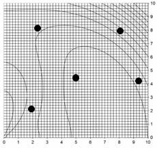
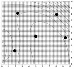
Figure 1: Leapfrog explanation step 1, initialization
My preference is leapfrogging (LF), a multiplayer direct search algorithm. Initially place many players (trial solutions) on the surface throughout feasible DV space. Determine the player with best, and with the worst OF values. Then move the worst player to the other side of the best player in DV space. The worst player “jumps” over the best player, like the children’s game of leapfrog, and lands in a random spot in the projected DV area on the other side. Hence the term leapfrogging.
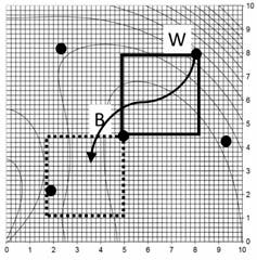
Figure 2: Leapfrog explanation step 2, choosing leap-to area
Figure 1 is an illustration on a 2-D contour, with a minimum at about 7.5 on the horizontal axis and about 2 on the vertical axis. Five trial solutions, five players, are illustrated with markers and are randomly placed over feasible DV space. Note: There should be about 20 players, 10 per DV, but only 5 are shown for simplicity of presentation.
Calculate the OF for each player; identify the worst and best. These are labeled W and B in Figure 2, which also shows the leap-from DV area (the window with the solid border) and the leap-into area (dashed border). The leap-to area is illustrated with the same size in DV space, but is reflected on the other side of B from W. Both window borders are aligned with the DV axes. W leaps to a random spot inside of the reflected DV-space window as the arrow indicates.
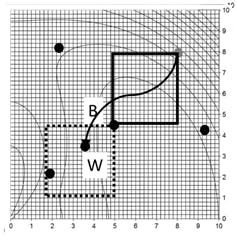
Figure 3: Leapfrog explanation step 3, the leap-over
The calculation of the new DV position is very simple. If there are two DVs, x and y, the leap-to location is calculated as:
Xw1new=Xb - rx(xw - xb)
Yw1new = Yb - ry(Yw - yb)
Here, ri are independent random numbers, with a uniform distribution and range of 0 < r ≤ 1. These random perturbations are independent for x and y. Note: The procedure scales to higher order, or to a univariate search.
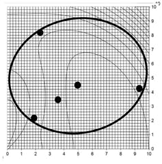
Figure 4: Leapfrom explanation step 4, test for convergence
As Figure 3 reveals, W moved to new position, and its prior location is vacated. Determine the OF value at the new player position. Note several features: The new position is not in the center of the leap-into window. There are still 5 players. All but one remain in their places. There is only one new function evaluation for the leaping player’s new position.
Test for convergence. As Figure 4 indicates the players are still far apart in DV space, as indicated by the size of the ellipse that contains them. They are not converged, yet. Any of many metrics can be used to determine when the players are all close to the optimum; but for presentation simplicity, I often use either average or root-mean-square deviation of all players from the best as represented in DV space. However, the range of the OF deviation from the best has advantages as a convergence criterion.
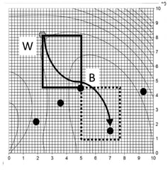
Figure 5: Leapfrog explanation step 5, next leap-over
Since the team has not converged, repeat the procedure. Identify B and W. In this illustration the best is still the best. The former worst now has a mid-contour value, so a new worst is identified. Note: If the leap-to spot was either infeasible (for any reason, an explicit DV constraint, a execution error in the OF evaluation, etc.) or had a worse OF value than the leap-from point, that player remains as worst. Also note: The leap-from and leap-to windows are not square.
In Figure 5, the new W leaps over B. One player is moved. Now the OF of the new location needs to be determined. In this illustration, the leap-to position is closer to the optimum, so the former W will become the new B.
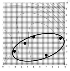
Figure 6: Leapfrog explanation step 6, test for convergence
In Figure 6, the team of players is both contracting and moving toward the optimum. The team is converging.
After repeating the steps, a few times, the players converge on the optimum.
Note: If there are N dimensions, each leap-over changes all N DV values for the jumping player.
Note: The TS values of this method are continuum-valued. But this can map to either discretized or class variables. Keep the continuum values for the player positions, but if feasible values are discretized values use nearest discretized values for the OF. If the DV is a class variable (such as PLC, DCS, SLC, PC) then allocate ranges of the LF DV to each class. For example, on a 0 to 10 basis if DV ≤ 2 the category is a PLC, if 2 < DV ≤ 4 then the category is DCS, etc.
Again, I believe this method is very simple to understand, has a low computational burden, has a high probability of finding the global optimum, and is not confounded by surface aberrations due to digital model methods (numerical striations, discontinuities, nonlinearities) and can naturally handle discretized variables, class variables, and even stochastic OF responses.
This explanation of leapfrogging optimization was extracted from my book Engineering Optimization: Applications, Methods, and Analysis, 2018, John Wiley & Sons, New York, NY, ISBN-13:978-1118936337, ISBN-10:1118936337. For free access to a detailed explanation of several optimization algorithms and demonstration software visit my web site www.r3eda.com.
Mark Redd has provided free access to open-source code in Python. Visit https://sourceforge.net/projects/leapfrog-optimizer/.

About the Author

R. Russell Rhinehart
Columnist
Russ Rhinehart started his career in the process industry. After 13 years and rising to engineering supervision, he transitioned to a 31-year academic career. Now “retired," he returns to coaching professionals through books, articles, short courses, and postings to his website at www.r3eda.com.
