Filtering a noisy signal

Noise can be viewed as random perturbations on an otherwise constant signal. If there were no noise, the signal value would remain unchanged. However, noise makes the signal fluctuate above and below the true value. Noise may be the result of mechanical vibrations, stray electromagnetic impulses, flow turbulence or any number of causes.

Further, the true value of the signal may be changing in time. The problem is that you can't see the true signal; all you can know is the noisy measurement or a calculated value. Figure 1 illustrates a slowly changing signal being confounded by noise. The true value of the signal is represented by the dashed line, illustrating that it's unknown. The control system can only know the fluctuating marker values, representing the measurement.

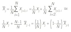
The problem is that noise confounds action. For example, between times of 19 and 21, the measurements seem to indicate a significant drop in value, while it's actually rising slowly. We would like to remove noise from signals, variables and action, and averaging is a common way to temper the fluctuation:

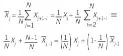
Here, the signal value is X, and the index j indicates the time. The index i is the counter for the 1st, 2nd…up to Nth past values that are to be averaged. Note that all N X-values need to be saved, and updated with each increment in time.

However, averaging wasn't possible with analog instruments of yesteryear, and even in the digital age, represents a computational burden of storing many N variables. Filtering is a computationally simpler approach to “averaging” and can be developed a number of ways.

Here is one: Take the most recent X-value out of the sum, and recognize that if the signal is not changing (at steady state), then the past average is a reasonable estimate for the sum.

Now all that has to be remembered is the past value of the average. The approximately equal sign reveals that even at steady state, the noise on the past average is different from the noise on the most recent, so the substitution of the average for the sum is not exact. Further, this substitution assumed that the signal is at steady state, which it may not be. Accordingly, don’t call this approximation the average, call it a filtered value. I’ll also rename the 1/N value as a filter factor, λ. The resulting equation is a first-order filter:

This equation is the digital representation of a resistor-capacitor circuit, or also a pneumatic tank-and-restriction device, used to temper noise. It's the numerical solution to the ordinary differential equation (ODE) of the RC circuit. Its mathematical form is also termed an autoregressive-moving-average of orders 1 and 1 – ARMA (1,1). The equation could be presented as its Laplace or z-transform version. Accordingly, there are many diverse representations for it, and you may find one or another classification names in the product bulletins of your devices. The variable λ may be indicated as the filter factor, f. Alternately, the value and complement may be reversed, so the (1-λ) term multiplies the most recent measurement. Still, the device might ask the user to choose the filter time-constant from which it would calculate λ=1-e(-Δt/τ). In any case, the user must specify the filter coefficient value; so, be sure that you understand which version your device is using.

[sidebar id =1]

The challenge for the user is choosing the right value for the filter coefficient. Filtering doesn't remove noise, it tempers it. So it would seem that more filtering (smaller λ value) is better to see the true signal. However, filtering induces a lag to Xf that masks the reality of an immediate change in the process. As filtering is increased to attenuate noise, the lag is also increased. The lag is undesired. It confounds the controller, and any other action that a person might take when observing a signal.

Figure 2 indicates the impact of three choices of filter coefficients on a signal that makes a step change to a steady value. The true, but unknowable, value is the dashed line, and the markers represent the data. Note that as filtering is increased, fluctuations on Xf are reduced, but the undesirable lag is increased.

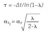
Ideal equations for the time-constant for the filter lag (obtained by numerical representation of the ODE) and the variance reduction (obtained by propagation of variance on the filter equation, assuming steady state and un-correlated noise) are:

One could desire a particular variance reduction, then calculate the required λ-value from one equation, and the consequential lag from the other. However, idealizations make the equations approximations; and more realistically, the filter coefficient will be heuristically adjusted online to meet a visual and subjective desire for noise reduction.

[sidebar id =2]

Since process noise amplitude changes with operating conditions (pH, nonlinear signal processing, flow turbulence and many other aspects), expect to readjust the filter coefficient value as changes in measurement signal would indicate. But also realize, the consequent significant changes in the time-constant could affect controller tuning.

Filtering may be effected on the process sensor, data transmission or controller. Be aware of choices that other technicians and operators may make. Tune the controller after the filter coefficient is set.

In filtering, the user needs to understand: 1) the balance of desirables (reduced fluctuation) and undesirables (increased lag); 2) the equation that the device is using; and 3) the impact that the lag may have on controller tuning and performance, and on the interpretation of the process by human observers.