Unveiling ancient global temperature and current climate change

In connection with my column, ”Heat balance of our planet” in the May issue of Control, readers asked about the reliability of the measurements of ancient global temperatures and today's global warming (GW) values because they amount to a temperature rise of only 1°C or 2°C per century. To answer, let’s look at the history of global temperature during the last 500 million years.
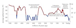
Figure 1 shows that the global temperature never dropped below 10°C or increased more than 30°C and that all the ice on the planet melted (red) when the global temperature increased to about 18°C (corresponding to a GW of 4°C). Therefore, all ice today will melt at 4°C, and at that point, ocean levels will rise by 66 m (216 ft). Figure 1 also shows that, until the Industrial Age, the global temperature was dropping (the planet was cooling), so warnings started only very recently. However, once the burning of fossil fuels started, global temperature started to shoot up at an unprecedented rate (about 1°C) during the last century. This rate of rise can only be explained by human activity, namely by the greenhouse effect of burning fossil fuels, resulting in the accelerated accumulation of CO2 in the atmosphere.
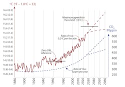
The rate of rise in temperature since 1960 was about 0.3°C per decade. This was caused by a rate of rise in the CO2 concentration of about 5 ppm per year. This concentration dropped during the COVID-19 pandemic, but it’s rising again. During the last million years, the CO2 concentration never reached 300 ppm. Today, it’s about 420 ppm.
The worst-case scenario can turn out to be even worse than what’s shown by the two dotted lines in Figure 2. This is because the U.N.'s limit of 1.5°C GW was already temporarily reached in July 2023, which was the warmest month ever recorded. I should also note that local GWs can be much higher than global averages. For instance, the average GW of land is almost twice that of the oceans, and the GW in the Antarctic is almost five times as much. In addition, local temperatures are also a function of the albedo (reflectivity) of the surfaces. For example, in cities without trees and with solar radiation-absorbing dark roofs, plus asphalt-covered roads and parking lots, the local temperature can be 10°C higher than elsewhere.
The reason why the predicted future values in the figure can turn out to be too low is because they don’t reflect the impact of delayed oceanic effects, albedo changes and the consequences of reaching any of the tipping points. Some of these effects will cause self-acceleration and/or positive feedback. It’s interesting to note that some of these effects can be counter intuitive. For example, an increase in GW reduces the heat conveyor effect of the Gulf current, where flow is larger than the sum of all river flows on the planet. This slowing is caused by the melting of ice in Greenland. It hasn’t started yet, but when it does, it will cool the northeast U.S. and northwest Europe. Similarly, the El Niña effect on the Pacific is already felt on the U.S. west coast, and is projected to intensify this winter. The time constants of these oceanic GW processes are much longer. Therefore, their effects are slower to evolve than the atmospheric ones, because the mass of the oceans is some 200 times greater than the atmosphere.
I already covered the accuracy of GW and CO2 measurements in my March 2020 and May 2020 columns. So, all I need to add is that, over the past century in the area of temperature measurement, we’ve gone from using mercury and alcohol thermometers to utilizing sophisticated satellite technology, artificial intelligence (AI) and other new technologies. Today’s GW data comes from more than 32,000 weather station, including weather balloons, radar sensors, ships, buoys and satellites.
Scientists working on estimating global temperature anomalies include groups at NASA (GISTEMP), NOAA (NCEI), Hadley Centre/Climatic Research Unit (U.K.) and Berkeley Earth. Despite using different methodologies in their research, they're all in close agreement on their conclusions. They cover different percentages of the Earth's surface, with NASA GISTEMP covering the largest area, more than 99%. Without going into the details on their methodologies and algorithms, I’d just mention that as extra heat is absorbed by our planet, the Earth's total heat content is rising. By measuring heat both in the oceans and on the land surfaces, GW can also be accurately calculated.
As to estimating ancient temperature and CO2 concentration values, methods differ depending on the time periods. During the last 1,000 years, for example, we know that between 1100 and 1300 A.D., the planet experienced a medieval warming period, while around 1600 A.D., the Little Ice Age occurred. The climatic fluctuations and temperature records of prehistoric times are reconstructed by indirect methods, using information such as tree ring widths, pollen grains, coral skeletons, isotope variations in ice cores and, from ocean or lake sediments, cave deposits, boreholes and glacier length records, which all correlate with climatic fluctuations.
Like tree rings, pollen production also largely depends on existing weather conditions. The abundance or absence can help establish how warm/cold the temperature was at a particular time. In the case of CO2, its concentration in the atmosphere can be determined from the isotopes and stomata on fossil leaves. Oxygen isotopes in deep sediments at the bottom of water bodies, such as the layers formed by the shells of small, surface-living animals that are deposited over millions of years, can also be used for such purposes. Although none of these techniques provide absolute results, they provide us with enough information to make educated guesses about the climate of the planet millions of years ago.
About the Author

Béla Lipták
Columnist and Control Consultant
Béla Lipták is an automation and safety consultant and editor of the Instrument and Automation Engineers’ Handbook (IAEH).
