Centrifugal pump control: Implications of high-static head/system pressure in VFD applications

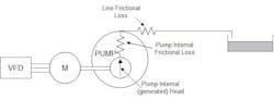
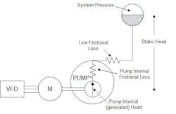
A little analysis of the hydraulic equations for the variable speed pump in the delivery of flow to the system can shed light on the reason for the distinct difference in behavior between flow control in systems where the pump delivers into a system with high system pressure and/or high-static head and when it is delivering into a low pressure system. Common examples of each of these systems are the high-pressure feedwater supply system for a power boiler and a low-pressure product pipeline. Figure 3 and Figure 6 show each system schematically.

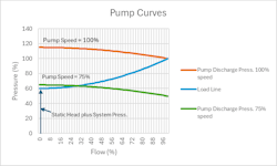
Figure 1illustrates the characteristics of a typical centrifugal pump delivering flow to a process operating at a high pressure, high static head or a combination of  pressure and static head that is high. The figure shows the pump discharge pressure as a function of flow for 100% pump speed and 75% pump speed. That the discharge pressure reduces as flow increases is due primarily to the internal frictional losses at the pump. The load line shows the pressure required at the pump discharge to establish a given flow with the pump operating against the combination of the static head and system pressure, and the frictional pressure drops in the line or process components. The pump flow is given by the intercept of the pump discharge pressure curve and load line.  Notable in this example is that the pump does not begin to deliver flow until the pump is operating at approximately 72% speed (when the pump internal head matches the combination of system pressure and static head) and that for just 3% increase in speed (to 75%) the flow increases by approximately 30%. On the other hand, increasing the speed from 75% to 100% increases the flow by 70%, illustrating the high variability in process gain and problematic rangeability discussed in detail below.

For the power boiler (without a feedwater regulating valve in this example), the pump must deliver enough head (proportional to speed squared) to overcome the drum pressure, the static head, the pressure drop in the economizer and evaporator (proportional to flow squared) and the pump internal pressure drop (proportional to flow squared). Before the pump delivers any flow at all, the pump internal generated pressure must match the system pressure plus the static head. In the example, with a system pressure of 1,000 psi and a static head of 44 psi (100 ft elevation difference between pump and drum), the pump wouldn’t deliver flow until it reached 82% speed (). It goes without saying that a non-return valve in the line is a must in this case.

For the control engineer, the difference in behavior are salient and in the case of the high pressure system, present a challenge in achieving high turn down with precise and stable control at lower flows.

Further analysis

The plot of the pump discharge pressure and load line (Figure 1) is often provided by the pump vendor for a specific application and is useful in predicting the operating point of the pump for a variety of loading conditions, however for analysis (and modelling) the mathematical representation  of the pump in-situ characteristics are more appropriate.

For the pump: P_d = k_ph * N² - k_pf * Q² (an approximation)

For the line: P_l = k_lf * Q² + P_s

Since P_d and P_l must match (are connected): k_ph * N² - k_pf * Q² = k_lf * Q² +P_s

Rearranging:

 Q = √(k_ph * N² - P_s)/(k_pf + k_lf)

It is also useful to derive the normalized equations for pump flow using the ratio of the system pressure (including static head) to the pump internal pressure at 100% flow (Φ). In this case, if the speed at which the pump delivers flow is N_min

N_min = 100 * √Φ

and the flow is given by:

Q = 100 * √(N²/10⁴ - Φ)/(1 - Φ)

For those who are interested, the derivation of this equation is given in the appendix.

Referring to equation (1), if P_S is the same as the pressure at the inlet of the pump, then Q is proportional to N. If this is not the case (in instances of high static head/system pressure), the relationship is not linear and can present a challenge in terms of resolution, turn down and controllability.

For the centrifugal pump, the developed head is proportional to the speed (N) squared, for a small change in speed (δN), the change in head (δP_p) is then proportional to N₀* δN (where N₀ is the initial speed). For the frictional pressure drop (pump internal pressure drop and line pressure drop) for a small change in pressure drop, the change in flow (δQ) is proportional to  δP_f /Q₀.  Since the change in pump internal head is balanced by the backpressure due to the frictional losses, by substitution, the change in flow (δQ) for a small change in pump speed is proportional to N₀ /Q₀ * δN.  Not surprising then, for the high pressure system, when the flow is zero and the speed 82% (in this example) before flow begins to increase, the process gain is very high (theoretically infinite) only then reducing as speed and flow increase.  For the high-pressure system, while the reduced speed range does not inherently (except for resolution) pose a challenge for control, that the gain at flows less than 30% increases significantly means that gain adaption is difficult to reliably apply. Since the system pressure can vary with load and the static pressure vary with load and temperature, the point at which flow is established by the pump varies and can add uncertainty to low load operation. Since in the high-pressure system, the effective range speed adjustment is low, the quantization of the analog output from the controller can have a greater effect on flow control in the high-pressure system than on the low-pressure system and that the D/A converter at the analog output for pump speed control should be 12 bit or more.

Table 1 illustrates the dramatic effect of the quantization of the speed demand value when derived from a digital/analog converter.

In Table 1:

Φ is the ratio of the flow independent downstream pressure i.e. system pressure plus static head, to the pump internal developed head/pressure at full (100%) flow. When the pump downstream discharge pressure is low e.g. the line discharges to an atmospheric tank or pond, Φ will be zero or close to zero. In the example used as a reference case for high static head or high system pressure, typical of a power boiler, Φ equals 0.7 (approx.)

N_min is the pump speed (%) that must be attained before the delivery of flow begins.

ΔQ₁₀ is the change in flow at 10% flow for a change in speed demand equivalent to a change in the least significant bit at the controller D/A converter.

ΔQ₁₀₀ is the change in flow at 100% flow for a change in speed demand equivalent to a change in the least significant bit at the controller D/A converter.

Table 1 is telling in that it indicates that, except in the case of a low-pressure line discharge, the resolution provided by 8 bit D/A is not high enough to provide any kind of precision in the control of flow. Also shown in the table is N_min which is the pump speed at which the pump first delivers flow. Since the entire range of flow adjustment is obtained from speed adjustment from N_min to N₁₀₀ it is not surprising that the precision of flow control (under speed adjustment) reduces as Φ increases. It will be seen later that torque control can improve linearity (and flow control precision) when Φ is greater than 0.2. Note that φ can never equal 1 since the pump would never overcome the system pressure to deliver flow, and that the closer φ approaches 1 the worse resolution becomes.

Model equations:

Induction motor:

T_M = (f - N) * 100/Slip_max

Pump flow (high static head/system pressure):

Note that in order to simplify the calculation of flow when the pump recirculation stream is modelled for pump minimum flow control, a node is created at the pump discharge and a mass balance calculated to allow for the calculation of pump discharge pressure by integration. This is equivalent to assuming (for convenience) that the fluid is slightly compressible.

Qp = √(0.1544 * N² - P_d)/0.02

dP_d/dt = Q_p - Q_R - Q_L

Q_L = √(P_d - 1044)/0.02

Q_R = 0.0127 * CO_R * √P_d

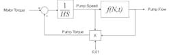
Pump acceleration: 

T_p = 100 * Power/N

T_p = 100 * P_h * Q/N * 100

T_p = N² * Q/ N * 100

T_p = N * Q/100

dN/dt = 1/H(T_M - T_p)

Hydraulic characteristics – low discharge head:

When the pump delivery line discharges to atmosphere or more precisely, at the same pressure as the pump inlet, the equation for flow (equation (1)) reduces to:

Q = √k_ph * N²)/(k_pf + k_lf)

Or:

Q = N√k_ph/(k_pf + k_lf)

In this case pump flow is linearly related to pump speed (Figure 4), and pump speed (or VFD frequency) the manipulated variable of choice for flow control.

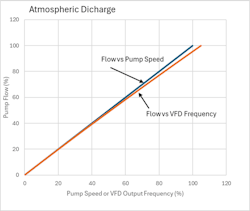
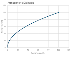
What then is the relationship between flow and motor torque for the low static head/system pressure discharge application ?

Referring to equation  (4) where pump torque is given by:

T_p = N * Q/100

For a pump discharging to atmosphere or pressure equal to the pump suction pressure, the flow is proportional to speed, and the normalized pump flow will equal 10 * √T.  Since this relationship (shown in Figure 5) is clearly non-liner, in this case, controlling pump flow by modulating pump torque by adjustment of VFD output current (and voltage) would offer a challenge in maintaining stability due to the variability in gain.  We will see later how the ratio of line discharge pressure to pump internal head at 100% flow in a particular application can be used to select the best method for flow control.

Hydraulic characteristics – high static head/discharge pressure:

When the pump is delivering to a high-pressure system or has to overcome a high static head, flow cannot begin until the pump delivers enough internal head to exceed the system pressure and or static head.  Figure 7 illustrates the relationship between pump speed and flow for an application where the modelled system pressure is 1000 psi, the static head 44 psi, the pump internal pressure loss 200 psi and 100% flow, and the line loss 200 psi at 100% flow. In this case the pump does not deliver flow until the pump speed is 85%, leaving only 15% adjustment for the control of flow. Note too, that the relationship between speed and flow is highly non-linear with very high values of process gain at low loads. Figure 8 plots calculated incremental gains δQ/ δN against flow to more clearly illustrate the non-linearity of process gain and the extreme gain variation at flows less than 10%.  Note that the gain at 5% flow is 57 (from raw data) and is 15 times higher than that at 100% flow. Interestingly, the plot of δQ/ δf against flow (Figure 9) is less non-linear at low flows due to the influence of induction motor slip on torque, to suggest that if torque control is not available (discussed later), directly modulating VFD frequency for flow control might be a better option than modulating frequency through a secondary speed control loop in a cascade strategy.

Get your subscription to Control's tri-weekly newsletter.

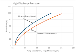
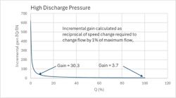
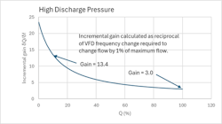
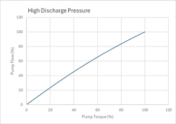
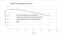
Figure 10 illustrates the relationship between pump flow and pump torque for the modelled high static head/discharge pressure application. Notable is the near linearity of the relationship, the incremental gain varying from 1.2 to 0.8 as shown in Figure 11, a factor of only 1.5. Also to note, is the fact that under torque control, since the torque varies from 0 to 100% as flow varies from 0 to 100%, turn-down is (theoretically) unrestricted, and the resolution for flow control determined only by the number of bits in the D/A converter and the process gain at a given flow.

A method for selecting the right control mode

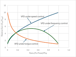
Comparing the variability of process gain over the load range for each of the three operating modes of the VFD (speed, torque or frequency), can aid in the selection of an operating mode for a particular discharge pressure /pump maximum internal head ratio. For this purpose, the gain at 10% flow and 100% flow is calculated for φ ranging from 0 to 1 (0 to 0.99) and the ratio plotted against φ.

Q/100 = √(N²/10⁴ * P_h100 - P_s)/(P_h100 - P_s)

Q/100 = √(N²/10⁴ - P_s/P_h100)/(1 - P_s/P_h100)

Q/100 = √(N²/10⁴ - φ)/(1 - φ)

Differentiating:

dQ/dN = (N/100)/√(1 - φ) * (N²/10⁴ - φ)

By calculating dQ/dN (the process gain for speed adjustment) at 10% flow and 100% flow for various values of φ and plotting the ratio (relative gain) against φ, the relative gain can be compared to that for the torque and frequency control modes to aid in the selection of the best performing control mode.                          

For torque:

T = N * Q/100

dT/dQ = N/100 + Q/100 * dN/dQ

dT/dQ = N/100 + Q/100 * dQ^-1/dN

dQ/dT = dT^-1/dQ

For frequency (for slip = 5% at 100% torque):

f = N + T * 5/100

df/dQ = dN/dQ + dT/dQ * 5/100

df/dQ = dQ^-1/dN + dQ^-1/dT * 5/100

dQ/df = df^-1/dQ

Referring to Figure 12, when φ is less than approximately 0.2 (pressure at discharge is less than one fifth of the pump internal head at 100% speed), the variability in gain with torque adjustment is greater than the variability with pump speed or VFD frequency adjustment,  and there is no advantage in applying torque adjustment for the control of flow in this case. When φ is greater than 0.2 there is a clear advantage in implementing torque adjustment for flow control. In the modelled reference case, which represents the feedwater controls on a power boiler, where φ is just over 0.7, for torque adjustment the process gain at 10% flow is just 1.5 times the gain at 100% flow a ratio that is so low that gain adaption may not be necessary. Flow control by the adjustment of VFD output frequency offers lower variability in gain over the range 10-100% compared to pump speed adjustment indicating that there is no material benefit in implementing closed loop speed control of the pump.

Valve differential pressure control by the adjustment of pump speed/VFD frequency

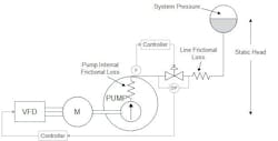
Figure 13 illustrates an alternative method for flow control where a valve is used for adjustment of flow and the differential pressure across the valve controlled at a fixed setpoint by adjustment of pump speed (or VFD output frequency). With constant differential pressure across the valve, with a valve with linear trim, the flow is linearly related to valve position. When the turn down requirements cannot be met by a single valve, a low load valve and main valve can be used in a conventional split range strategy to provide a high turn down ratio. Because the valve differential pressure is constant and is low, valve wear is much reduced compared to applications where the pump speed is fixed and the valve is subject to a high pressure differential al low load. Although the pump speed range of adjustment is not improved but is slightly lower than the range for flow control without a valve, the resolution in speed does not affect the precision in flow control but does introduce a small uncertainty in gain at any operating point.

Dynamic Model Results-system without flow regulating valve

Open loop response variation with load:

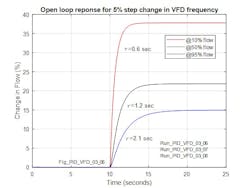
Figure 14 shows the response for a step change in VFD output frequency, at 10%, 50% and 100% flow for the High system pressure/high static head case. For the same step change in frequency the flow change is higher at low flows than at higher flows but the process gain at each load would appear to be lower than that suggested in Figure 9, and the gain variation lower over the load range. This is due to the change in frequency (and flow) being higher than that used the static calculations.  Notable in the response is the fact that the response time is shorter at lower loads, which is contrary to the trend with typical processes and is attributable to the increase in stabilizing feedback ΔQ/ΔN at lower loads. Figure 2 may help with this deduction.

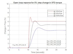
In Figure 15, for a step change in torque the response is underdamped since in this case the negative feedback due to the influence of slip on motor torque is absent. It should be noted that a step in torque would not ordinarily occur in practice due to the response of the VFD under torque control but that the response of the modelled system is indicative of the inherent response of the motor and centrifugal pump.

Flow control

The model implements PID (series) controllers for process flow control by adjustment of the VFD setpoint and for pump minimum flow control, adjustment of a recirculation valve at the pump discharge. The PID controllers implement integral action through filtered positive feedback which allows controller output limits to be implemented to be simply implemented. Controller derivative action is filtered so that the high frequency gain of the derivative term is limited to 4. The controller and process model execution rates are independently adjustable to allow for the realistic behavior of the digital controller. The model includes quantization of the controller output, and for the presented cases assumes 12-bit D/A conversion. The VFD response (in the frequency demand mode or torque demand mode) is modelled by a rate limit, a 1 second deadtime and 5 second lag time. The model implements the previously described pump/motor inertial and flow equations. The reference dynamic model for the cases with direct adjustment of the VFD (frequency or torque) adopts the same static head (44 psi) and system pressure (1000 psi), and same line and pump internal pressure drops at full flow as used in the reference case for the steady state calculations. As such φ is approximately 0.7, which suggests (according to Figure 12)  that torque control of the VFD would be the preferred strategy.

Flow Control - VFD in frequency demand mode

In this mode, the controller output determines the frequency demand for the VFD. That the process gain varies so much over the load (flow) range for the pump requires that the controller gain be adapted so that it reduces as flow reduces. Table 2 shows the control parameter settings for the flow controller when the VFD is in the frequency demand mode.

Figure 16 shows the response at 10% flow when the flow setpoint is increased by 5%. Note that due to the high process gain, Just discernable, is the limit cycle on speed (and flow) due to the quantization of the frequency demand signal from the controller. It should be born in mind that the performance of the VFD in terms of the minimum step in frequency adjustment also affects the precision of flow control, and that this must be considered in the selection of equipment.

Figure 17 shows the response at 10% flow when the flow setpoint is reduced by 8% to just 2%. In this case the pump minimum flow controller is in Auto to serve to adjust pump recirculation (or return to sources) to maintain minimum pump flow at 10%. Forward flow to the system (for instance power boiler drum) is reduced to 2% without interaction with the minimum flow controller. More noticeable in Figure 17 is the limit cycle due to the quantization of the controller output which with a 12-bit D/A converter would be .07% pk to pk but with an 8-bit D/A converter would be 16 times greater or over 1% pk to pk.

Figure 18 shows the response at 10% flow when the flow setpoint is reduced by 8% to just 2% when the pump minimum flow controller is in Manual. Although operating in this condition is inadvisable, the case does show that operating at such low loads requires great precision in frequency control since an 8% reduction in flow requires only  0.15% change in pump speed.

Flow Control - VFD in torque demand mode

When the VFD is in the torque demand mode, the output of the flow controller is forwarded to the VFD is the setpoint for torque. The VFD response to the torque demand is modelled by a rate limit, deadtime and a 5 second lag. In this mode, the model dispenses with the torque slip equations since the motor torque is regulated by the VFD. Other than these differences, the model is identical to that used in the response assessment with the  VFD acting in the frequency demand mode, with process conditions replicating the high static head/system pressure application. For these conditions, φ is approximately 0.7 and torque control is recommended according to Figure 12.

VFD operation in the torque demand mode for pump flow control is distinguished by an unrestricted range of adjustment (see Figure 10 above), and for the modelled high static head/high system pressure application, little process gain variation of the load range (see Figure 11).

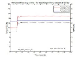
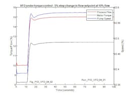
Figure 20 shows the response for a 5% step in flow setpoint at an initial flow of 10% with the VFD in the torque demand mode. For this low load optimized gain and reset are 1.75 and 7.5 seconds respectively. Noticeable in the response is the absence of any signs of a limit cycle due to the quantization of the flow controller output since, with an effective torque adjustment range of 0-100, the minim step for torque adjustment (and flow approximately)  is 0.024%.  

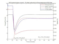
Figure 21 shows the response for a 7% step reduction in flow setpoint at an initial flow of 10% with the VFD in the torque demand mode. In this case, the minimum flow controller is in Auto and reacts to maintain pump minimum flow at 10%. Intuition might suggest that since the pump torque is dependent on the total pump flow (process flow plus recirc flow), there might be interaction between the flow controller and minimum pump flow controller, however this is not the case, with the difference in loop response times a contributing factor.

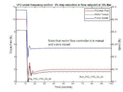
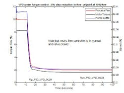
Figure 22 shows the response at 10% flow when the flow setpoint is reduced by 7% to just 3% when the pump minimum flow controller is in Manual. Although operating in this condition is inadvisable, the case does show that despite the fact that the flow is still ultimately adjusted through a torque induced speed change and the flow highly sensitive to speed at low loads, stability at low flows is more easily achievable when the VFD is operating in the torque demand mode.

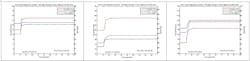
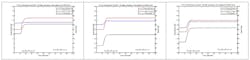
Figure 23 shows the response for a 5% increase in setpoint at 10%, 50% and 95% flow when the VFD is operating in the torque demand mode. Significant here is the fact that the response at each load is obtained with the same gain and reset (1 and 5 seconds respectively), only possible  in this operating mode when there is little variation (according to Figure 11) in process gain over the entire load range.

Behavior overload range (Flow controller-process gain=1, IAT = 5 sec)

Dynamic model results-system flow regulating valve

For the system shown schematically in Figure 13, the hydraulic model is only slightly adjusted to provide additional pump head to account for the pressure drop across the valve. Here, the controllers are repurposed to adjust valve position to control flow and VFD output frequency to modulate pump speed to maintain the valve differential pressure at 100 psi. In this case, the pump minimum flow controller (recirc valve) is not modeled.

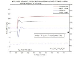
Figure 24 shows the response at an initial flow of 10% when the flow setpoint is stepped to 15%. Notable in this case is that the speed has only to increase by 0.2% (frequency by 0.4%) to maintain 100 psi across the valve at the higher valve opening. Less noticeable in this case is the ripple on the flow due to the quantization of the controller output by the D-A converter since it manifests as a limit cycle on the valve DP rather than directly on flow.

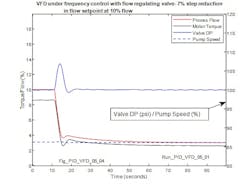
Figure 25 shows the response for a step reduction in flow set point at 10% initial flow to a very low 3% flow. It is optimistic to assume that a single valve would have this high range of turn down, however, the control range can be increased by implementing a split range strategy involving two or more valves with the valve differential pressure across the valves controlled by pump speed (VFD frequency) adjustment.

Figure 26 shows (for comparison) the closed loop response at loads 10, 50 and 90% for a change in flow setpoint with the flow controller acting on the valve and valve differential pressure maintained by adjustment of the VFD demand frequency. The response may be directly compared to that shown in Figure 19 for flow control by direct adjustment of VFD demand frequency. Understandably, since flow control using a valve requires the cooperative action of two controllers, one controller acting on the valve and the other controller acting on the VFD, the response is slower in this case but does offer the opportunity for high turn down in flow by adding a low load/start-up  valve if necessary.

Conclusions

The drive for efficiency and the lowering of operating costs has encouraged the adoption of VFDs for the control of motor driven centrifugal pumps. Overlooking the in-line characteristics of the centrifugal pump can easily lead to an over specification of the VFD control provisions and add unnecessary cost or under specification to create operational challenges.

 For applications where flow is controlled by the direct adjustment of the VFD, broadly speaking, for high static head/process pressure applications the more complex torque demand mode is recommended for flow control. Using the variability of process gain as one metric for choosing a control strategy, if the ratio of (Ps+Pstat)/ Php is greater than 0.2 (approximately), then it is better that the VFD operate in the torque demand mode.  A power boiler is just one application of many that fall into this category. For high static head/process pressure applications, operating the VFD in the speed or frequency demand mode results in a reduced range of adjustment at the controller and in such applications demands a high resolution at the controller output and the implementation of adaptive gain with an order of magnitude gain adjustment in some cases.

For applications where (Ps+Pstat)/ Php is less than 0.2, for instance when the pump is delivering to an atmospheric tank or pond, speed or frequency control is favored although there seems little advantage in adding the complexity of closed loop speed control unless useful for feedforward control particularly when there is not a flow controller. There is little additional burden on practitioner if the speed control is implemented in VFD and tuned by the VFD supplier. The extremely fast execution rate of speed control in VFD eliminates any concern about violation of the cascade rule where there primary process controller in the DCS or PLC must be at least five time faster than secondary speed controller.

Although not presented here, it is useful to consider the startup of the pump with the VFD in the torque demand mode. With only mechanical friction resisting the acceleration of the pump, a small torque demand will accelerate the pump until the speed is high enough to start delivering flow. When flow is established, flow control can be transferred to Auto. Any concern regarding the possibility of the pump over speeding if there is a restriction in the flow can be resolved by the addition of a speed override implemented in the VFD or DCS 

More on good practice:

1. Use input and output chokes and isolation transformers to prevent EMI from inverter.
2. Use PWM to reduce torque pulsation (cogging) at low speeds.
3. Use inverter duty motor with class F insulation and 1.15 service factor and totally enclosed fan cooled (TEFC) motor with a constant speed fan or booster fan or totally enclosed water cooled (TEWC) motor for high temperatures to prevent overheating.
4. Use a NEMA Design B instead of Design A motor to prevent a steep torque curve.
5. Use bearing insulation or path to ground to reduce bearing damage from electronic discharge machining (EDM) that is worse for the 6-step voltage older drive technology.
6. Size pump to prevent operation on the flat part of the pump curve.
7. Use a recycle valve with an independent flow controller to control pump minimum flow.
8. Use a non-return valve to prevent reverse flow at the pump during startup or shutdown.
9. Use at least 12-bit controller output cards and ideally 16-bit VFD input cards to improve the resolution.
10. Use drive and motor with a generous amount of torque for the application so that speed rate-of-change limits in the VFD setup do not prevent changes in speed being fast enough to compensate for the fastest possible disturbance.
11. Minimize dead band introduced into the drive setup, causing delay and limit cycling.
12. For tachometer control, use magnetic or optical pickup with enough pulses per shaft revolution to meet the speed resolution requirement.
13. For tachometer control, keep speed control in the VFD to take advantage of the typically higher execution rate in the VFD to prevent cascade rule violation where the secondary speed loop is not 5 times faster than the primary process loop.
14. Use external reset feedback of accurate and fast speed readback to stop oscillations from poor VFD resolution and excessive dead band and rate limiting.
15. Use foil braided shield and armored cable for VFD output spaced at least one foot from signal wires with never any crossing of signal wires, ideally via separate cable trays.