Key Highlights
- Not all process noise behaves the same. Asymmetric noise can bias measurements, autocorrelated noise violates the assumption of independent data points, and signal discretization can create false impressions of steady-state conditions.
- Filtering isn't always the answer. While filtering can smooth noisy signals, it may introduce measurement bias, increase lag or even create autocorrelation.
- Better data leads to better control decisions. Selecting appropriate sampling rates, identifying outliers correctly, and understanding the effects of sensor resolution and transmitter filtering can improve controller tuning, statistical process control and confidence in process performance analysis.

Noise may not be ideally symmetric as upward perturbations may have a different amplitude from downward perturbations. This might be due to pressure pulses in a flowline because small ones are larger than large ones, or due to a nonlinear feature such as square root extraction of sensor values or a statistical distribution of perturbations that puts a long tail on one side of a distribution. If the perturbations are not symmetric, filtering will shift the reported average toward the larger amplitude side, creating a bias and confounding even steady state analysis.
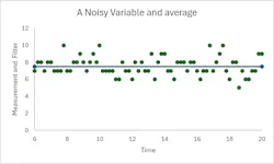
There are several visual characteristics of asymmetric noise. During a steady state period, the negative deviations are clearly farther from (or nearer to) the average, and there will be more data on one side of the average than the other. Figure 1 reveals both departures from ideal. During the steady period 10 to 20, there are more markers above the filtered value than below, and the below markers are generally farther from the average than the above markers.
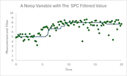
The problem is that it creates a bias on the measurement—the average is pulled toward the more extreme data. The distortion from symmetric data violates the assumptions about normally distributed data that are the basis for statistical analysis, such as t-tests or variance estimation. If the noise level is relatively small or the disparity between plus and minus deviations is not excessive, the nonideality can be usually ignored. If there is copious data at steady state, which does not have symmetric noise, the median (the 50-percentile value) will be a better representation of the true process value than the average.
Autocorrelation
Noise is generally considered to be perturbation additions to the true measured value, which are independent at each sampling. Something real causes the perturbation. If that something persists in the next sampling, it will have a similar impact on the next measurement. What this means is that if a prior measurement is on the high side, then the next measurement will likely be high also. Both measurements are contaminated by the same event. These persisting influences cause autocorrelation in the perturbations. Sequential perturbations are not independent.
As an example of a mechanism causing autocorrelation, clouds passing by the sun might be randomly causing changes in solar energy hitting your process, which affect internal temperatures. But the clouds don’t blink on and off at the frequency of your data sampling. Both cloud cover and clear periods persist for a brief duration, so the sequence of temperature measurements will progressively rise and fall.
As another example, batch-to-batch raw material feed causes composition changes that persist for a duration.
Finally, at-sensor filtering to temper noise or the sensor lag caused by a thermowell both cause autocorrelation. There are many sources of autocorrelation.
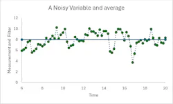
Figure 2 illustrates autocorrelation during a steady period. The dashed connect-the-dots line helps visualize the trend in the data values. If one point is high, then next will likely also be high. If one is low, likely so will the next. The trend is like oscillation, but the above and below periods are not regular in either amplitude or duration. Unlike asymmetric noise, the number and range above the average is about the same as below.
Another way to detect autocorrelation is to plot one data value with respect to the prior data value. If there is no autocorrelation, the pattern will be circular. If there is autocorrelation the data pattern will be an oval with an upward or downward trend. The term “Lag-1” means that the data sequence is shifted by one, which is what Figure 3 represents.
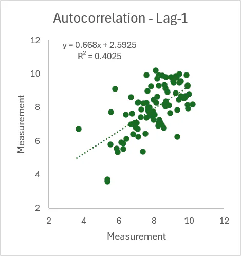
Although the correlation trend is visually obvious, one could do a statistical test on the R2 correlation coefficient to support an autocorrelation claim.
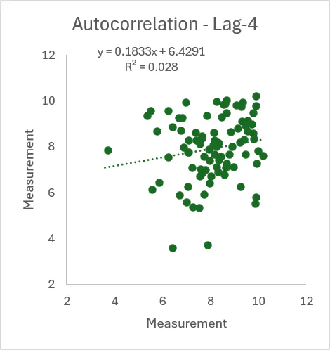
Figure 4 indicates that at Lag-4 (one data point plotted vs. the fourth prior point) no autocorrelation is visible. In this simulation, the impact of influence on the fourth past data point has faded enough so that it does not have a noticeable impact on the most recent measurement.
Autocorrelation might be the result of pulsing in piston pumps, on-off level or temperature control, unit switching for regeneration, changing properties of raw material feed, BTU content of a shovel-full of coal, or process device issues such as stick-slip (sticktion) in a valve. It may appear to be random noise on a less frequent sampling interval, but normal measurement frequency can track the persisting ups and downs making it look like the real trend, which it represents.
Similarly, external environmental influences on the process can cause perturbations that have persistence. Consider wind gusts, rain showers, or passing clouds that create intermittent cooling of external units, which persist for a brief time. Again, the persistence of these on-off disturbances will cause temporary measurement changes with autocorrelation.
Filtering also causes autocorrelation. Filtering is a form of averaging, and each measurement persists in the averaging window, until time passes it out. Or, in the case of a first-order filter, in which the influence is exponentially weighted by time, the influence of all past data remains in the calculation, but after enough samplings the exponential weighting make the past perturbations inconsequential.
The controller can cause autocorrelation. If a step disturbance pushes the process off of setpoint, the controller begins changing the manipulated variable, until the integral action accumulates enough to move the controlled variable to the set point. The deviation persists until fixed.
Instead of using the instrument and control system to cover-up (filter) or to control the persisting perturbation, eliminate the source. For example, improve feed material blending, use pulse dampers, or put positioners on valves. Alternately, reduce the sampling frequency so that the short-term persistence has faded prior to the next sampling. However, reducing sampling frequency may cause a delay in sensing process changes.
Many statistical tests are based on the no-autocorrelation assumption. These include t-tests on differences, steady state detection, and statistical process control charts. Although you might want a controller to work on a high frequency, you also might want to use less frequent sampling in process analysis to remove autocorrelation from the data.
Because the manufacturer designed a controller to operate at a 10 Hz frequency, doesn’t mean it is better. An old rule of thumb is that there should be 30 actions in a settling time. If your process has a 20-second time-constant, the 95% settling time is roughly 60 seconds, and a control frequency of 0.5 Hz should be adequate. If there is perturbation autocorrelation at the high sampling frequency, it might disappear at the lower, but still fully adequate, rate.
The high value of one sampling does not cause the high value of the next. There is a third variable that persists for a while, which affects sequential measurements similarly. Filtering at the sensor/transmitter may have been chosen by someone installing or calibrating it to generate a smooth signal. You may want to reconsider the filter tuning.
Outliers are not noise
Relative to a control system, errors that should be ignored are missed/dropped signals or other spurious signals such as those due to electromagnetic pulses from motor startups. Median filters are a sensible solution. In a middle-of-three filter, the middle value of the last three signals is accepted as the representative value. If one signal is absurdly high or low, one of the other two will have the middle value. The middle value might be the most recent, the second past, or the third past. On average this will cause a delay of one sampling as the reported value. If you think a spurious or outlier event might have a persistence of three sequential signals, use the middle of the past five measurements.
Methods to remove outliers (infrequent spurious events that should be rejected) are different from those intended to reduce noise by filtering data. Using a first-order filter strong enough to render the outlier inconsequential probably will cause an undesirably significant lag.
Resolution
Signal discretization can give an appearance of noise. Discretization can come from many sources such as digital transmission devices or analog-to-digital display. This is like the digital time display when seconds or minutes jump from the past value to the present, then hold that value during a time interval until it jumps to the next. However, for a process signal that is progressively drifting about a value, signal discretization generates either a flatline hold until enough change makes it jump, which is a false indication of a noiseless steady state, or a square wave signal that seems to randomly jump between certain discrete values (with no in between values).
The visible clue to signal discretization is that the signal jumps between certain values (Figure 5.) Note the lines of dots with identical values, and no dots with in between values. If a process is nonlinear, the discretization may have very small intervals (not noticeable) in one range, but large enough to be visible in another range.
I would not label this discretization signal as noise; however, filtering could minimize its amplitude (but also introduces a lag). To eliminate the appearance of noise due to signal discretization, use higher bit converters.
All digital devices have discretization. If an instrument is calibrated for a wide PV range, the discretization interval on the reported measurement will be large, and possibly visible. Consider calibrating over a smaller PV range.
This is part two of a three-part Develop Your Potential series. Read part one here and part three here.
About the Author
 R. Russell Rhinehart
R. Russell Rhinehart
Columnist
Russ Rhinehart started his career in the process industry. After 13 years and rising to engineering supervision, he transitioned to a 31-year academic career. Now “retired," he returns to coaching professionals through books, articles, short courses, and postings to his website at www.r3eda.com.
 Leaders Logo
Leaders relevant to this article: