Energy correlation method: Measuring mass flow with differential pressure flowmeters

Prior to discussing differential pressure flowmeters, my Industrial Flow Measurement seminar students are asked to choose whether orifice plates are simple or complicated devices. Almost everyone raises their hands for simple but not one for complicated. What do you think? 

The consensus answer is correct. Not so fast! Ask why and you will find that users have the work performed by others. Here, the manufacturers of flow elements perform precise calculations to fabricate and calibrate the flowmeter. Simple. However, further investigation will reveal that the calculations themselves are complicated. 

The discharge coefficient for differential pressure flowmeters is proportional to volume flowing through a pipe. The Buckingham equation used to calculate the orifice plate discharge coefficient was developed using data generated from orifice plate studies at Ohio State University Engineering Experimental Station in the 1930s. Some of this data was later used to develop the Stolz equation, which was adopted in International Organization for Standards (ISO) standards in 1980, whereas the American National Standards Institute (ANSI) continued to use the Buckingham equation. 

Data from a study performed by the American Petroleum Institute (API) in the 1980s was used to resolve discrepancies between the Buckingham and Stolz equations. The resulting Reader-Harris / Gallagher equation, shown immediately below, was adopted by both ISO and ANSI in the 1990s. Note its complexity, dependence on Reynolds number, minimum pipe diameter of 50 mm (2-inch), and minimum Reynolds number of 10,000. 

C = 0.5961+0.0261β²-0.216β⁸

+0.000521(10⁶β/Re_D)^0.7

+(0.0188+0.0063A)β^3.5 max{(10⁶/Re_D)^0.3, 22.7-4700(Re_D/10⁶)}

+(0.043+0.0080e^-10L₁-0.123e^-7L₁)(1-0.11A)β⁴/1-β⁴

-0.03 ](M₂-0.8M₂^1.1){1+8max(log₁₀(3700/Re_D), 0.0)}β^1.3

+0.01 ](0.75-β)max(2.8-D/25.4,0.0).   (D : mm)

Equations in ISO 5167 can be manipulated to yield the following proportionality relationship describing the mass flow through a differential pressure flowmeter. A similar proportionality for the flowing volume (not shown) can be obtained by dividing both sides of the mass flow relationship by g*w.

Q_mass ∝ (C*ℇ(Y)*d²_bore/√1-β⁴)*√∆P*g*w

where: Q_mass is the mass flow of fluid

C is the discharge coefficient, which is the ratio of actual flow to ideal flow through a restriction

ℇ(Y) is the expansion factor (for gas applications)

d_bore is the diameter of the bore

β is the ratio of the bore to the diameter of the pipe

∆P is the measured pressure drop across the restriction

g is the acceleration of gravity

w is the specific weight of the flowing fluid

The discharge coefficient C and the expansion factor ℇ(Y) are individually derived from experimental data or estimated from theory. In practice, the discharge coefficient is dependent on the geometry and size of the flow element, beta ratio (β), and the pipe Reynolds number, which itself is a function of flow, density, viscosity, and pipe diameter. ℇ(Y) for liquids is unity (1) but for gas applications, ℇ(Y) is dependent on the beta ratio (β), ratio of specific heats of the gas, upstream pressure, and the differential pressure across the flow element. Determining the values of the variables mentioned in this paragraph introduces complexity and measurement uncertainty. 

This all seems complicated (and it is), but it is relatively easy to implement for most applications by having the flow element manufacturer perform detailed calculations using process information provided by the user. However, this approach assumes that the user possesses complete and accurate process information, which is often not the case. Custody transfer and flow laboratory applications that usually involve fluids with known physical properties can incorporate flow computers programmed to perform precise calculations and achieve better accuracy. 

For the last 100 years or so, differential pressure flowmeter standards, research and everyday industrial process flow measurements focused on first measuring the flowing volume, and then correcting for operating conditions, such as by compensating for pressure and temperature. The focus on measuring the flowing volume is visible in the common use of mass flow measurement units that contain descriptions of volume, such as standard cubic centimeters per minute (sccm), as opposed to actual units of mass, such as kilograms per minute (kg/min). Stated differently, using differential pressure flowmeters to measure mass flow was largely an afterthought. 

Energy correlation method

In general, flowmeter technology, applicability and performance can improve via a combination of hardware, software and theoretical advances. For example, the performance of time-of-flight ultrasonic flowmeters can be enhanced with more powerful sensors. However, using the same sensors with different equations that do not include the speed of sound in the liquid removes a significant source of uncertainty, and can improve accuracy. Similarly, upgrading magnetic flowmeter electronics from sinusoidal to pulsed DC excitation dramatically improves accuracy from a percentage of full scale to a percentage of rate while still using the existing magnetic flowmeter sensor. 

During the initial months of the COVID-19 epidemic (2020-2023), Zaki Din Husain, Ph.D theorized that differential pressure flowmeters could be used to measure mass flow and subsequently derived the following mass flow proportionality using his Energy Correlation Method.

Q_mass ∝ (d²_bore/√1-β⁴)*√∆P*g*w

Comparing Equation 1 and Equation 2 reveals that the latter equation replaces C * ℇ(Y) with a linear function obtained from experimental data. Notably absent are the discharge coefficient C, expansion factor ℇ(Y), and therefore, a dependency on Reynolds number, which simplifies calculations and removes multiple sources of uncertainty. Independence from these intermediate parameters and their respective constraints can enable differential pressure flowmeters to be used in applications that previously would not have been considered. 

It should be noted that differential pressure flowmeters manufactured to tolerances specified in a standard will produce the same differential pressures under the same operating conditions regardless of which flow equations are used to calculate the flow rate. Therefore, the Energy Correlation Method can be applied to any differential pressure flowmeter geometry. 

However, the salient question is whether the Energy Correlation Method relationship can be used to calculate mass flow, and if so, how accurately it performs as compared to equations presented in standards. 

These questions can be answered by calibrating differential pressure flowmeters as mass flowmeters using the Energy Correlation Method and then evaluating their performance. A more pragmatic approach is to apply the Energy Correlation Method to existing differential pressure measurement mass flow data and similarly evaluate performance. Examples illustrating both approaches follow. 

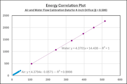
Air and water flow laboratory calibrations

Flow laboratory calibrations of a proprietary differential pressure orifice flow element were performed in air and water. Recorded data included the differential pressure produced by the flow element, fluid density, mass flow rate, pipe Reynolds number, and discharge coefficient. Since the influence of the local acceleration due to gravity is captured in the density of the flowing fluid between the location of the calibration facility and the location in which the flowmeter is operated, the acceleration due to gravity (g) can be removed from Equation 2. 

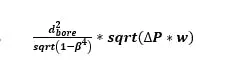
Figure 1 is the plot of the calibration data, where the X-axis values are (d²_bore/√1-β⁴)*√∆P*g*w and the Y-axis values are the corresponding values of the mass flow rate. The linear best-fit lines for the air and water data are displayed with their respective slope, zero intercept and R2 values (coefficient of determination or goodness of fit). 

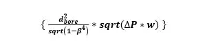
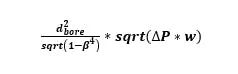
The term (d²_bore/√1-β⁴)*√∆P*g*w is the Energy Correlation Function. The mass flow rate measured by this calibrated flowmeter when installed in the field, at any differential pressure measurement and corresponding fluid density is,

Q_mass = slope * (d²_bore/√1-β⁴)*√∆P*w + zero intercept

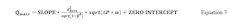
where the slope and zero intercept values capture the influences of (π*√2*g/4). Note that the dimensional units of the Energy Correlation Function plot of the calibration data for actual installations must be consistent with the dimensional units of all the variables in Equation 2.

For example, if the differential pressure reading and the density value at given flowing conditions generates an energy correlation function {(d²_bore/√1-β⁴)*√∆P*w} value of 450, the slope and zero intercept values in Figure 1 can be used to calculate the mass flow rate of that fluid as (4.3701 x 450) + 14.438, or 1981 flow units, which approximately corresponds to the second data point from the right in Figure 1.

Observation of Figure 1 in conjunction with its calibration data reveals:

• R² values describe the “goodness of fit”, where R² values of 0 and 1 indicate low and high correlations of the data, respectively. Hence, the R² value of 0.9998 for this data indicates a high correlation of the data. 
• This flowmeter measures mass, so the slope and zero intercept values can be obtained from a flow calibration in any fluid. Further, the same slope and zero intercept can be used to measure the mass of any other fluid flowing through this flowmeter.
• The value of the slope times the energy correlation function (X-axis value) should be greater than 10 times the value of the zero intercept to achieve accurate flow measurement.
• The value of the zero intercept accounts for the influences of the flow rate measurement uncertainties of the calibration facility, flow profile distortions, and the effects of fluid property variations.
  • The zero intercept value of the air calibration data exhibits a negligible contribution to the calculated flow rate (under 0.15 percent), which supports the general validity of the Energy Correlation Method.
  • The water intercept exhibits a larger effect (under 3 percent) that possibly results from increased measurement uncertainty at differential pressures that are low in the transmitter range.
  • The small difference between the air and water slopes (0.21 percent) implies that the mass flow rate measurement is virtually independent of fluid state which supports the general validity of the Energy Correlation Method.

Get your subscription to Control's tri-weekly newsletter.

American Petroleum Institute (API) flow laboratory calibrations

The discharge coefficient and Energy Correlation methods can be illustrated using API natural gas flow calibration data sets that were collected in the 1980’s to establish a flow equation for orifice plate flowmeters and to determine straight run requirements for various upstream piping configurations. The flow equation was established using approximately 7000 of the 10,000 sets of data collected. Some data sets were discarded to develop the flow equation because their installations were intentionally designed to not comply with the standards that were subsequently developed from the data.

Figure 2 is a traditional plot of the discharge coefficients as a function of pipe Reynolds number for 4-inch orifice plates having four (4) different beta ratios and various upstream piping configurations, including those that did not comply with standards.

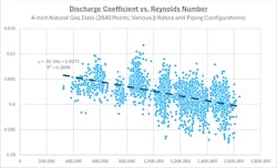
By observation of Figure 2:

• The curve fit R² value implies a relatively poor correlation of the data.
• The discharge coefficients vary from the fitted curve (dashed line) by over ±1 percent, which is understandable given the inclusion of installations that did not conform to standards. 
• The fitted curve (dashed line) slopes downward by approximately 1 percent over its 6:1 range of Reynolds number. 

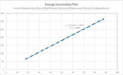
Figure 3 shows the same calibration data sets as Figure 2 as an Energy Correlation plot exhibiting a linear relationship and superior curve fit R² value. Further, Figure 2 and Figure 3 contain many data points that are not in conformance with installation standards. Therefore, the superior R² value in Figure 3 shows that the Energy Correlation Method exhibits improved immunity to installation effects.

Additional calibration data sets

Energy Correlation plots performed by Dr. Husain produced similar linear relationships for the following data sets.

• API liquid and gas orifice plate flowmeter calibration data containing different meter sizes, beta ratios, and piping configurations, including orifice plate flowmeter calibration data from Gas Unie (The Netherlands) and Gas de France (France) that were later added to the API database.
• 2-inch to 20-inch Venturi flow meter calibration data, including bidirectional Venturi flowmeters
• 2-inch orifice plate flowmeter water calibration data (0.1 and 0.05 beta) operating in the laminar, transitional, and turbulent flow regimes where the slope value was the same in all flow regimes
• Drilling muds with significantly different densities (12, 14, 16, 18-pound mud) and viscosities operating in the laminar, transitional and nearly turbulent flow regimes

Energy Correlation Method advantages and disadvantages

Application of the Energy Correlation Method can affect many aspects of differential pressure flow measurement. 

Measurement of flowing volume

Differential pressure, magnetic, positive displacement, turbine and vortex shedding flowmeters infer volume, measure volume, or measure velocity. In general, the ubiquitous availability of these flowmeters gave rise to the practice of specifying measurements in units of flowing volume. 

In contrast, the relationship obtained by dividing both sides of Equation 2 by the specific weight (not shown) enables the Energy Correlation Method to measure the flowing volume. 

Mass flow measurement

Mass flow measurements are usually more beneficial than flowing volume measurements. It is possible, but cumbersome, to compensate inferred volume, measured volume, and fluid velocity measurements for actual process conditions, such as operating pressure and operating temperature. Therefore, viable mass flowmeter technology options are limited.

• Coriolis mass flowmeter technology is widely applied because it uses the properties of mass to measure mass. 
• Thermal mass flowmeter technology applications are limited to the measurement of gases (typically with known composition) and are sensitive to heat transfer properties that can vary significantly with operating pressure, operating temperature and composition. 

The Energy Correlation Method enables differential pressure flowmeters to measure mass flow in a wide variety of applications, including applications for which differential pressure flowmeters would previously not have been considered. 

Applicability

The Energy Correlation Method enables widespread application of differential pressure flowmeters while simplifying calculations, potentially improving accuracy, and relaxing multiple constraints, as will be discussed. 

Accuracy

Dr. Husain verified that the Energy Correlation Method conforms well with the API orifice plate flow laboratory calibration data. Investigation of other data sets indicates that the Energy Correlation Method can be used to determine the slope and zero intercept values for any differential pressure flowmeter. 

Operation at low flow rates

Differential pressure flow transmitter accuracy is typically a fixed differential pressure, often specified as a percentage of calibrated span. Therefore, its accuracy as a percentage of flow rate degrades as the actual flow rate drops. Extracting the square root of the signal increases degradation. 

For example, a differential pressure flowmeter operating at 20 percent of full-scale flow rate will produce only 4 percent of its full-scale differential pressure (0.20 * 0.20). A transmitter accuracy of 0.05 percent full-scale means that its output should be between 3.95 and 4.05 percent, which corresponds to an accuracy of approximately 0.63 percent of the actual flow rate. Similarly, the accuracy is approximately 2.5 percent of the actual flow rate at 10 percent flow. By observation, flow accuracy at low flow rates is dominated by transmitter performance and not by a primary element. The accuracy degradation at low differential pressures can be mitigated (when required) by installing an additional lower-range differential pressure transmitter in parallel to more accurately measure the low differential pressures generated at low flow rates. 

The previous paragraph is generally valid for custody transfer and flow laboratory installations that conform to standards. However, almost no differential pressure flowmeters used to monitor and control industrial processes conform to standards due to a lack of knowledge, cost or both. 

Sensitivity to installation

The Energy Correlation Method exhibits superior immunity to installation affects, so it is likely that straight runs can be shorter than currently specified in standards. Shorter straight run requirements enable more compact and less expensive installations in custody transfer and flow laboratory installations. Installations used to monitor or control flow in industry can exhibit better accuracy at the same cost, despite their non-conformance to standards. Existing API flow laboratory calibration data can likely be used to quantify the straight runs necessary for accurate measurement using the Energy Correlation Method. 

Calibration

Differential pressure flowmeters using the Energy Correlation Method are mass flowmeters. Therefore, they can be wet calibrated using any fluid within constraints, such as high viscosity (discussed below). It is likely that the API flow laboratory calibration data can be used to determine the slope and zero intercept values for standard differential pressure flowmeter geometries. 

Errors associated with the magnitude of the differential pressure can be ignored when the ratio of the differential pressure between the upstream and downstream pressure taps to the upstream line pressure is less than 5%. 

Sensitivity to density (specific weight)

Coriolis mass flowmeters use the properties of mass to measure mass and are not affected by fluid density variations. Thermal mass flowmeters are unaffected by gas density variations per se, but can be affected by temperature, pressure and composition. 

Mass flow measurements derived from magnetic, positive displacement, turbine and vortex shedding flowmeters are affected by density changes such that measurement of the same mass flow with a 1 percent higher density will cause the mass flow derived from the flowing volume measurement to be low by 1 percent. Differential pressure flowmeters inherently have superior immunity to density changes because they exhibit approximately half of this effect due to their square root extraction. Regardless of flowmeter technology and calculation method, density measurements can be used to compensate for these effects to improve accuracy when required. 

Sensitivity to Reynold Number and viscosity

Measurements using the Energy Correlation Method are not directly affected by Reynolds number, per se. However, the differential pressure produced by the same mass flow through a differential pressure flowmeter using the Energy Correlation Method is not significantly affected when the amount of kinetic energy measured is much larger than the combined pressure losses due to pipe roughness, flow profile distortions, and fluid viscosity. Increasing fluid viscosity can eventually cause significant friction losses that affect the measurement. Testing should be performed to quantify viscosity constraints.  

Flow computers

Flow computers are often not necessary because the slope and zero intercept calculations can be configured in differential pressure transmitters or other external devices. 

Cost considerations

Cost can play a major role in flowmeter selection. Every application is different; however the cost of thermal flowmeters (where applicable) often falls in between less expensive differential pressure flowmeters and more expensive Coriolis mass flowmeters. 

Summary

The Energy Correlation Method is not dependent on Reynolds number, discharge coefficient, expansion factor, or viscosity (within constraints) and fits the API flow laboratory calibration data used to develop the Reader-Harris / Gallagher equation. Independence from these variables simplifies calculations, reduces sources of uncertainty, and enables differential pressure flowmeters to measure mass flow in a wide variety of applications, including applications where they were previously not considered. 

Calibration can be performed in any fluid to determine the slope and zero intercept for the flowmeter at flow rates that need not correspond directly with the specified flowmeter range. Therefore, large flowmeters need not be calibrated near their full-scale flow rates, but rather at lower flow rates that are easier to implement. In addition, the relatively simple calculations can mitigate the need for flow computers. 

The Energy Correlation Method has been submitted for inclusion in both API and ANSI (via ASME) standards.