Control strategies improve solar plant efficiency
Key Highlights
- Simulation allows safer control strategies testing.
- Digital twins help quantify control improvements, estimate economic benefits, and troubleshoot processes
- Digital twins require substantial engineering effort and must be calibrated and validated with plant data.

The Plataforma Solar de Almeria, Spain, is a full-scale CIEMAT research center for exploring several approaches to generate electricity from thermal collection of solar energy. CIEMAT (Centro de Investigaciones Energéticas, Medioambientales y Tecnológicas) is a Spanish public research organization focused on energy, environment and technology.
An aerial view of the TCP-100 facility (Figure 1) shows its parabolic trough collection (PTC) approach. Mirrors in the parabolic trough refocus sunlight on a pipe that runs along the mirrors’ focal points. Oil is heated as it runs through the pipe, and the hot oil is used to generate superheated steam to run a turbogenerator.
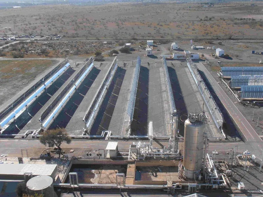
There are three lines that loop north and then south in the TCP-100 facility. Each line has a total collection length of about 96 meters. The mirrors change orientation during the day as they track the sun. Direct normal irradiance (DNI) is the intensity of solar energy falling on the aimed mirrors, and nominally increases from about 400 to 1,000 W/m2 and back to 400 W/m2 during the course of the day, though this value is also affected by local atmospheric events (mainly clouds). There are some ambient losses in each line, which depend on random changes in wind and ambient temperatures. For many reasons (fouling, dirt, mirror damage, sun angles, mirror aim), the optical efficiency of each line is unique and changes over time. Similarly, fluid friction loss factors change independently in each line due to changes in fouling and other inline effects.
Variable speed pumps feed return oil to the header for the solar collection lines. Valves in the lines adjust flow rates to make the exit temperature match a target, and pump speed is also adjusted to minimize parasitic power losses.
Currently, solar thermal plants have low levels of automation, largely because complex control systems that would demonstrate improved efficiency haven’t been developed. The results shown here are from a CIEMAT study on the TCP-100 Solar Collection facility.
One challenge is temperature control in the thermal collection line due to long and variable transport delays (2 to 5 minutes), nonlinearities, and continual uncontrolled input disturbances. Another is minimizing pump power consumption (parasitic losses).
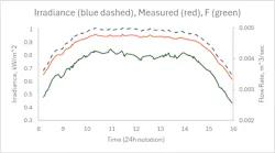
Figure 2 shows how DNI changes during a nominal day (with the solar peak at noon). Perturbations in the DNI trace (dashed line) are due to random walk perturbations driven by Gaussian noise. (See references 2 or 3 below for the applicable models.) The drifting influences were calibrated to mimic actual field measurements. Since we don’t know the absolute truth about what’s occurring in nature, we measure process variables. However, measurements have calibration errors, so the information that the controller has isn’t the true DNI. Instead, it’s the somewhat erroneous measured value, which is the middle trace in Figure 2. Ambient heat losses, inlet oil temperature and pipe friction factors, each have individual characteristic drifts and measurement errors.
Objective and strategy
The main control objective is to keep the exit oil temperature at a setpoint. As DNI changes during the day, so must the oil flow rate, which is the lower trace in Figure 2. The perturbations on it are larger than what the DNI alone would suggest because of simulated variations in ambient losses and inlet temperature.
The initial control strategy investigated by the authors was simple proportional-integral (PI) feedback on the exit oil temperature measurement and feed-forward correction based on the measured inlet oil temperature. It worked acceptably for the conditions it was tuned for (without significant variations in the DNI, inlet T or ambient losses). But, as the day progresses, the flow rate creates about a 2:1 change in the delay, and the process gain also has about a 2:1 ratio. Gain scheduling seemed to be a possible solution, but the number of scheduling factors for each of the 6 PI and FF tuning coefficients seemed to violate the keep it simple, stupid (KISS) principle.
The authors next investigated using a nonlinear feedback controller on the exit oil temperature (T) cascading a flow rate setpoint to a nonlinear flow controller. The T controller used generic model control (GMC) with a steady-state model. This is equivalent to classic advanced regulatory output characterization3. The model in GMC includes feed-forward compensation for the inlet T. The primary GMC temperature controller sent a setpoint value to the secondary model-based flow controller (MBC), which uses a simple, dynamic model for the flow rate response to the signal sent to the valve. This strategy is relatively simple, with only two tuning coefficients for GMC and one for MBC. It kept the exit temperature within ± 1 oC of the setpoint during the simulated day.
Midline temperature would provide an early indication of the impact of disturbances (inlet T, DNI and ambient losses) on the exit T. This suggests another level of cascade control. In this strategy, the exit T controller sends a setpoint to the mid-line T controller, which sends a setpoint to the flow controller that operates the valve. Since midline T is nearly a linear indication of exit line T, we used a PI controller for the exit T, cascading to the GMC controller for the midline T, cascading to the model-based flow controller. In total, there are five tuning coefficients, and over the simulated day, control kept the exit T within ±0.3 oC of the setpoint. This is an advantage because precise T control permits operating close to constraints for oil degradation and boiler performance. However, in this case, the improvement in net power that could be generated by operating 0.7 oC closer to a constraint is within the noise on power due to the process input variations.
Get your subscription to Control's tri-weekly newsletter.
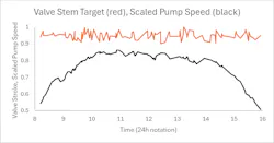
Finally, we the authors explored a supervisory adjustment of pump speed, with a simple logic to adjust speed to keep valves at about 95% open to minimize parasitic energy loss. If the pump remains at full speed during the day, then the valve must throttle flow rate to control temperature. This requires greater pump power than is necessary. By reducing pump speed if the valve is less than 92% open and increasing pump speed if the valve is more than 98% open, the valve is kept at about 95% open. This provides some immediate control flexibility, while minimizing parasitic losses. Figure 3 shows how the signal to the valve and pump speed (as a fraction of maximum) change during the simulated day. Compared to operating the pump at 100% speed during the day, this action reduces parasitic losses by about 25%, which is significant.
This example reveals that simulation can be used to investigate alternate control strategies, quantify the reduction in controlled variable variation, and quantify the resulting economic benefit (in this example, operating power consumption.)
Perspective
The domain of control engineering is more than control algorithms. It includes the instrument system, process optimization, dynamic and steady-state simulation, calibration, design, equipment selection, coding, device communication, and standards for each.
Develop your potential in all aspects of the profession to add value as a control engineer. Use simulation to explore and quantify the economic benefits of improved control.
Simulators aren’t free. They can consist of phenomenological models that range from rigorous to first-principle types. They could include empirical models for some elements of the process. They could be steady-state design models adapted to represent dynamics with simple linear dynamic add-ins. In any case, digital twins require engineering effort to create, update as processes changes, and validate against process data. Once you have a digital twin, however, it serves many other engineering endeavors, such as process troubleshooting, inferential process monitoring, design, personnel training, preservation of mechanistic process knowledge, and, of course, process control.
Acknowledgements
I greatly appreciate input on this article from Sandeep Lal, senior process control and optimization engineer at Chevron Phillips Chemical Co. LP. I also enjoyed collaborating with Luis J. Yebra of the CIEMAT Research Centre on simulation and control projects supported in part by the Spanish Ministry of Science, and the European Union. These projects include “Digital twin analysis of solar, parabolic, trough-collector plant to scale to higher powers for integration into electrical distribution network (DISOPED),” reference number PCI2022-134974-2, and “Modelling and diagnosis of parabolic trough collectors (MODIAG-PTC),” reference number TED2021-129189B-C21/TED2021-129189B-C22.
References
[1] Rhinehart, R. R., “Adding realism to dynamic simulation for control testing,” Control, Sept ’24, p. 33
[2] Rhinehart, R. R., “Adding realism to dynamic simulation for control testing,” Control, Oct ’24, p. 30
[3] Rhinehart, R. R., Nonlinear, model-based control: using first-principles models in process control, International Society of Automation, Durham, N.C., 2024
About the Author

R. Russell Rhinehart
Columnist
Russ Rhinehart started his career in the process industry. After 13 years and rising to engineering supervision, he transitioned to a 31-year academic career. Now “retired," he returns to coaching professionals through books, articles, short courses, and postings to his website at www.r3eda.com.

Leaders relevant to this article: